Connecting the Tech Stack: 5-Minute Interview with Tim Ward, CEO at CluedIn

June 29, 2018, 12:00 am

≫ Next: Machine Learning on Graphs: 5-Minute Interview with Ajinkya Kale, Senior Applied Researcher at eBay

≪ Previous: Detecting Fake News with Neo4j & KeyLines

Read this interview with Tim Ward, CEO at CluedIn, about using Neo4j for machine learning and more

“Connected data is always more interesting than disconnected data, especially when you’re wanting to do something like we do,” said Tim Ward, CEO at CluedIn.

For Tim, it’s all about flexibility, scalability and resilience. As the CEO (and an engineer) at CluedIn, he needed a primary data store to join together a tech stack with a variety of databases. With a graph database, Tim was able to automatically join vast and deep amounts of data and scale right along with a major company growth spurt that went from 15 customers to a database of 280 million nodes with close to a billion relationships in the graph.

In this week’s five-minute interview (conducted at GraphConnect New York) we discuss how Tim’s company uses Neo4j to enhance their polyglot tech stack design with new engineering techniques, including machine learning.

Talk to us about how you guys use Neo4j at CluedIn.

Tim Ward: My background is mainly in engineering. I’ve been a software engineer for 12 years, and I try different platforms out. And that’s really what brought us to Neo4j – it was different type of technology that was worth investigating.

At CluedIn, we take a very polyglot persistence design to our technology stack. We actually use a whole variety of different databases, and the way that we use Neo4j is actually as our primary data store.

It’s really based off this ethos that we have, that connected data is always more interesting than disconnected data, especially when you’re wanting to do something like we do, where we’re integrating data automatically from different systems.

It requires this kind of database where context, graph theory itself and the design patterns that are in it are really just necessary for solving this problem to a higher precision than the other types of technologies we are used to.

What made you choose Neo4j?

Ward: So I started working with Neo4J close to six years ago, and I started on an early 1.5 release. I think the interesting reason we were looking in the graph space was because of the new possibilities in engineering techniques it gave us.

Graph technology allows us a different data structure that solves problems that inherently other data stores you would typically bend to solve the same problem.

The three main points why we chose Neo4j were: first, its ability to join across huge amounts of data, no matter the kind of depth of the connection. The next was the pattern matching techniques and, finally, it was actually the kind of path traversals, the ability for us to kind of take two discrete nodes that were in our graph and to reverse engineer the connections between those two data points.

Neo4j, of course, for us, when we were looking in the market, it just seemed like the obvious choice. It had a fantastic company behind it. It had a lot of growth. It had some funding, which we knew that that technology could get the necessary attention that needed to fulfill the graph tech story.

So I think that and the combination of it integrating well with our stack and having the APIs available for us to work with it in an agnostic way, no matter what libraries we were using or languages, really helped – it was an easy choice for us to choose Neo4j.

Can you talk to me about some of your most interesting or surprising results you’d had while using Neo4j?

Ward: I think the most interesting results that we’ve had was our scale story.

We started off with 15 customers and grew our company into a database of 280 million nodes right now with close to a billion edges (or vertices) in the graph.

What surprised us, and that also challenged us, was the resilience behind the platform and, that being a generic graph model, you could really take control of the platform in the parts where potentially focus was needed from the product.

Especially around things like indexing and scaling using a schema instead of – we went through this era in the NoSQL area where no schema was something that was sold as a big plus. And what you really realize when you go to production is that, well, a schema is actually something that’s extremely necessary.

In Neo4j, our ability to influence how the core platform actually works with things like indexing, it was the flexibility that surprised us in a very positive manner.

If you could start over with Neo4j, taking everything you know now, what would you do differently?

Ward: I think what we realized after time is that there are some odd things that you might need to do with your model to cater for some of these scalability type of complexities and, to be honest, only really show themselves when you are in production at huge concurrent read and write levels.

You’re also dealing with such a diverse amount of data that’s not necessarily fitting all into the same model. We work with different customer data, and one customer’s industry looks completely different to the data from another industry.

The ability to have a model where, at a later point, we could bend and change, I think that was one of the things we would probably revisit. But in hindsight, maybe we wouldn’t have discovered that if we didn’t go with our original easy way of modeling the data.

What do you think the future of graph technology looks like in your industry or sector?

Ward: We’re on a very similar mission to Neo4j. We’re wanting to connect the enterprise, and we’re using a lot of the same techniques that Neo4j is also saying is in their vision. So, we’re using machine learning techniques as well.

Where we see the market going is that a lot more people are adopting graphs as just one of the extra types of databases you use to solve problems. And I think where it’s going is the application of machine learning, combined with things like the graph, to be able to produce results where companies actually start to utilize their data.

Companies can become data-driven. We can get out of these archaic ways of manually integrating systems in a very tedious, manual approach and move towards a company’s data telling us how things are connected.

In the future, maybe models for the graph will be inferred from the data instead of the other way around. I’d like to see if that’s where we’ll go.

Anything else you want to add or say?

Powers: It’s been great to talk to the people from the Neo4j product team and give them feedback from the field.

There’s huge value in being able to talk to the actual engineers changing those things, who make a tangible impact on allowing companies like us to be able to scale to some of the biggest companies in the world. I think that’s kind of priceless.

Want to share about your Neo4j project in a future 5-Minute Interview? Drop us a line at content@neo4j.com

Want to build awesome projects like this?
Click below to get your free copy of the Learning Neo4j ebook and catch up to speed with the world’s leading graph database technology.

Get the Free Book

↧

Machine Learning on Graphs: 5-Minute Interview with Ajinkya Kale, Senior Applied Researcher at eBay

July 6, 2018, 12:00 am

≫ Next: Decyphering Your Graph Model

≪ Previous: Connecting the Tech Stack: 5-Minute Interview with Tim Ward, CEO at CluedIn

Learn how Ajinkya Kale, Senior Applied Researcher at eBay's New Product Development Group, uses Neo4j.

“Most people are not yet looking at graph databases from a machine-learning point of view. All the inherent knowledge we as humans use to make decisions can be encoded in a graph structure,” said Ajinkya Kale, Senior Applied Researcher at eBay’s New Product Development Group.

For Ajinkya, it’s all about the synergy between graphs and machine learning. As a Senior Applied Researcher at eBay’s New Product Development Group, Ajinkya and his team use Natural Language Understanding to bake machine learning into the graph database that drives eBay’s virtual shopping assistant, eBay ShopBot.

In this week’s five-minute interview (conducted at GraphConnect New York), Ajinkya tells us how he got started with Neo4j and about his vision for machine learning on knowledge graphs.

Talk to us about how you guys use Neo4j at eBay.

Ajinkya Kale: We built eBay ShopBot using Neo4j as a probabilistic graph model to drive conversations. Conversational commerce is basically a system where you interact with the agent as you would interact with a salesperson in a shop, and so we needed to encode human understanding into our knowledge graph.

You’ve been using Neo4j a while, right?

Kale: I have been in the research field for almost five years now, and actually I have used Neo4j since I was working on my master’s.

There’s a funny story I told Emil. On one of my master’s projects, I was stuck on some issues. At that time, Peter Neubauer – one of the founders – was still at Neo4j. I posted on the Neo4j forum, and Peter just jumped on and said, “Hey, let’s do a Skype call,” and I said [laughing], “Okay, fine.” We shared screens and he fixed some things for me, which is pretty cool, having a founder get on a call with you.

What made you choose Neo4j?

Kale: We looked at a bunch of graph technologies. Neo4j’s track record and my experience with it were among the reasons we went with Neo4j as a graph solution.

Other factors were the ease of use, especially as a developer who is new to Neo4j, as well as the way you can visualize the data and play with it at the same time. From the experimentation phase to production, it’s super easy to use.

What do you think the future of graph technology looks like?

Kale: Most people are not looking at graph databases from a machine-learning point of view. All the inherent knowledge we as humans have accumulated since our childhood, the knowledge we use to make decisions, can be encoded in a graph structure. And that’s going to be a big thing going forward.

Want to share about your Neo4j project in a future 5-Minute Interview? Drop us a line at content@neo4j.com

Level up your recommendation engine:
Learn why a recommender system built on graph technology is more powerful and efficient with this white paper, Powering Recommendations with Graph Databases – get your copy today.

Read the White Paper

↧

Decyphering Your Graph Model

October 17, 2018, 12:00 am

≫ Next: Vampire Express: Graphing a Classic ’80s Choose Your Own Adventure Story

≪ Previous: Machine Learning on Graphs: 5-Minute Interview with Ajinkya Kale, Senior Applied Researcher at eBay

Watch Dom Davis' presentation on how to decypher your graph model.

Editor’s Note: This presentation was given by Dom Davis at GraphConnect Europe in May 2017.

Presentation Summary

Graphs really are everywhere, and building your graph database model from the highest possible vantage point using natural language – and the language specific to your domain – helps you develop a model that truly stands the test of time.

Full Presentation: Decyphering Your Graph Model

In this blog, we’re discussing how to develop the best graph model for your particular domain from the highest possible level:

At the startup Tech Marionette, we’re building the next generation of configuration management databases. This is backed by Neo4j because the assets in an enterprise don’t live in silos of a relational database. They’re interconnected graphs. And graphs really are everywhere! It’s not just a catchy marketing slogan.

Finding graphs is easy, but modeling them is the fun part. Most basic texts on graphs start with vertices and edges:

Learn how graphs start with vertices and edges.

From there, we dive off into graph theory. That said, making the leap from the world of numbers and letters into something slightly more useful isn’t that hard. And being a property graph with Neo4j, we can embellish our data with some useful stuff.

But jumping straight into Cypher isn’t necessarily the best way to go about discovering the model of your world.

Building Your Model Using Natural Language

A graph is essentially a way of modeling the world using interconnected triples in the format of noun-verb-noun. Take the below example, graphs (noun) are (verb) everywhere (noun):

It’s just English. The astute among you may notice there are countless other languages out there, many of which don’t follow this particular format. But we can make this work for any language regardless of the order of subject, verb and object. You simply reason about your model in your natural language and then map it back to the subject-verb-object field graph when you’re done.

Building a Natural Language Model in Your Domain

If you’re going to model the world, let’s start with the nouns of that world. If I was going to model this conference, we might start with the nouns below:

Discover how natural language processing workings for a graph model.

Taking our nouns, we can then form sentences with verbs:

Learn how natural language processing works by connecting verbs to nouns.

We’re creating a model that we can reason about because it’s using natural language. And once we have our nouns and our verbs, we have labels and relationships. The graph model just falls out nice and easy:

See an example of Cypher natural language processing for a graph model.

Now we can start embellishing our data. A “speaker” has a name, and the phrase “has a” implies a property. “Room” also has a name, and “talk” has a title and a start time – but does it have an end time? Or does it have a duration?

This really comes down to the question you’re going to be asking of your model. Questions like “How long did I spend in talks?” and “How long did I spend giving talks?” are possibly better answered with a duration, because it’s an easier calculation. But a question like “Will I be out of talk A in time for talk B?” may be easier with an end time.

We could put “company” and “roles” as properties of the speaker, but someone could have multiple roles at different companies. Also, “speaker has role at company” looks very much like verbs and nouns. Not only that, but “delegate has role at company,” too.

So let’s build these as part of the model, not tucked away inside properties.

Now we have the basis of a model that we’ve developed using language that’s easily understood, even by people who aren’t familiar with Cypher or Neo4j. This allows you to speak with these domain experts and build your model using natural language.

From Model to Graph

There are some considerations you need to take into account when you convert your model into a graph. While our verbs made sense of our nouns, we’re now viewing the world as instances of those nouns:

While “speaker has role” in our model made sense, “Dom Davis has CTO” doesn’t work in English, which shows that the semantics of our model didn’t survive the translation into the graph world.

I’ve highlighted another potential issue by having “role” as a one-to-many relationship, which requires the speaker-to-role relationship to be one-to-one.

To understand why, we need to look at a slightly different data set:

Learn about what a flawed graph model looks like.

Person (blue) has role at company (green). Because director (yellow) has many relationships in and many relationships out, with this particular model, it’s impossible to tell who is the director of which company.

Instead, we need to have an unambiguous route or path for us to follow with the below, Model A:

But this isn’t the only way we could have modeled the data. If we just care about companies and company directors, Model B might actually be more sensible:

Data-wise, Models A and B are pretty much the same. Although Model A is more flexible, having hundreds of different relationships between roles is not a good design.

We can store properties like “start dates” on the role, as well as on the “has_director” relationship, but we can’t index those properties and they are extremely inefficient to search. Relationship properties are really only there to help you make a traversal decision, or to give you data once you’ve made that particular traversal.

If you’re going to search on relationship properties, that’s a sign you may need to stick them in a node — even if adding extra nodes into the model may be an alien concept. But unless you have an atomic node and an atomic relationship with no properties, your graph could always be described with more nodes.

Diving Into Cypher

While (:Speaker {name: "Dom Davis"}) can also be written as (:Speaker)-[:HAS_NAME]->(:'Dom Davis'), let’s consider the “speaker-has-role” path in determining which works better:

For my conference profiles, I needed to include a primary role that could be dropped into my bio. We could tag this in our relationship with the “has role.”

But wherever you see this particular construct…

… you can also replace it with a specific relationship type:

You can also record it as a new node, which in this case has something coming off the role:

The abundance of ways to describe things within the graph is why you really want to drive the model with the language of the domain, not from the Cypher query.

If you consider the graph model that I’m working with, we have the idea of concepts, properties and relationships. This might sound like one-to-one mapping with nodes, properties and relationships in the graph, but it’s more complex than that. I have no idea how many properties a particular concept may have, and I have no idea what they’re going to be called.

Hopefully, we all agree that the below setup is absolute madness:

And while this next example is more extensible, I don’t want to see the query plan for things like “find me all the concepts with a ‘name’ property:”

Instead, we looked at how we described the domain. Concepts have properties, so while “has a” implies a property on a node, “has many” implies relationships and nodes.

The solution is the following, which effectively defines property nodes using property nodes and relationships (which is all very meta):

And then below this, we have the idea of instances, which have values:

So we’re defining a schema on our graph and then storing data under that schema.

In fact, we even have a schema node, which lets us do some really interesting stuff in our meta-model. Because the concepts defined in our model can called different things by different people, we can include the idea of “aliases” and “primary language.” You can then define aliases on that model and start asking questions using the terms you would naturally use.

Take a ticketing system for example. You could talk about any ticketing system you’d like, such as Jira or Bugzilla, and each ticketing system could have tickets, issues or tasks. All you have to do is add the aliases:

Conclusion

While the building blocks that Neo4j provides are simple, they’re also incredibly flexible and powerful. In the preceding example I’ve used them to model something that’s very basic, but which in itself lets you model something quite complex.

Have I just reinvented the wheel? No, because when we came to model the domain, we weren’t talking about ticketing systems. We were talking about arbitrary concepts — schemas, concepts, properties, relationships, instances and values — with properties and relationships between them. These were my nouns as I was discussing the domain.

We shouldn’t ignore what the language of the domain is telling us. If we wrote our model at the level of labels, nodes, relationships and properties as our nouns, we would continually have to change our queries and extend our query library every time the model changed.

When we use our model with more arbitrary concepts, it provides us with two models to describe and reason about: the meta-model. The meta-model is mostly complete and static, while the new model is evolving. And we reason about it using the same type of language, and the same advice applies because it really is just graphs all the way down.

Want to learn more about graph databases and Neo4j? Click below to register for our online training class, Introduction to Graph Databases and master the world of graph technology in no time.

Sign Me Up

↧

Vampire Express: Graphing a Classic ’80s Choose Your Own Adventure Story

February 21, 2019, 12:00 am

≫ Next: Graph Algorithms in Neo4j: Graph Algorithms in Practice

≪ Previous: Decyphering Your Graph Model

Check out this data model on a choose your own adventure series.

Here at Neo4j, we have a motto: Graphs Are Everywhere. This blog series was inspired by all the times I encountered graphs and “graph problems” in my non-working life. Hopefully these posts help you see more graphs in the world. If you’d like to share graphs you find in the wild, leave a post on the Neo4j community site, or send me a tweet (@joedepeau).

I’m a child of the ’80s. While I can look back now and recognize how naive, weird and downright cheesy much of the decade was, I still feel a strong sense of nostalgia when I think of certain things from my childhood. One pop culture phenomenon I fondly look back on is the Choose Your Own Adventure series of books.

Ten-year-old me couldn’t get enough of them: I read every single one in my school’s library, borrowed them from my friends and annoyed my parents until they bought me some of my own.

A very thoughtful friend gave me an original set of three mint condition Choose Your Own Adventure books for my most recent birthday. I devoured them pretty quickly and – looking at them from my adult point of view – I recognized something new right away: These stories form a graph.

In fact, I started to wonder how the authors mapped them out and kept track of everything during the creative process. Obviously graph databases didn’t exist back then (we’re talking 1984 here, they didn’t even have Excel), but if it had been me, I’d have gotten a huge piece of paper and drawn it out as what we now call a graph model.

Then I watched Bandersnatch (Netflix’s interesting “choose your own adventure” interactive show about a “choose our own adventure” game), and saw that’s pretty much what the main character did. That guy could really have used a graph database!

I decided to have a bit of fun, and load up one of my Choose Your Own Adventure books into Neo4j Desktop so I could see how graphy it really was. I selected Choose Your Own Adventure #31, Vampire Express by Tony Koltz, ©1984 by Metabooks, Inc. and Ganesh, Inc.

It only took about an hour or so to create a graph representing all the possible paths in Vampire Express. I used a very simple data model, with Pages represented as nodes and each Page node linked to the next by NEXT_PAGE relationships.

Some pages in the book simply point you directly to the next page in the story, and others present you with two or more options.

Where there are more than one options for the next page I created multiple NEXT_PAGE relationships from that Page node, and put the text for the choices into “option” properties on the relationships.

I also gave the first page an additional Start label, and each ending page an additional End label, so we know where the story begins and ends.

The “metagraph” or “data model” for this graph looks like this:

Using this simple model I was able to map out all the pages, choices and endings in Vampire Express. The full graph for the book looks like this:

Vampire Express as a graph, with the Start in green and possible End results in red.

Pretty neat, right? Ten-year-old me would have loved this graph stuff (especially if there was a driver for BASIC).

Using my graph and a few Cypher queries, I can answer some useful questions about this particular Choose Your Own Adventure:

Q: Are there any “loops” in the story that take you in a circle back to where you started?

In Cypher:

MATCH path = (s:Start)-[:NEXT_PAGE*1..]->(s)
RETURN path

A: No, there are no circular paths in this adventure.

Q: Are there any pages not reachable from the first page?

In Cypher:

MATCH (p:Page), (s:Start)
WHERE NOT (s)-[:NEXT_PAGE*1..]->(p)
AND p <> s
RETURN p

A: No, every page can be reached via a path from the first page.

Q: What is the shortest path to an End page from the first page?

In Cypher:

MATCH path = (s:Start)-[:NEXT_PAGE*1..]->(e:End)
WITH collect(path) as paths, collect(length(path)) as lengths
UNWIND paths as p 
WITH p WHERE length(p) = apoc.coll.min(lengths)
RETURN p

A: The endings on page 46, 87 and 107 can all be reached in seven “hops” (or page turns) from the first page.

Q: What is the longest path to an End result page from the first page?

In Cypher:

MATCH path = (s:Start)-[:NEXT_PAGE*1..]->(e:End)
WITH collect(path) as paths, collect(length(path)) as lengths
UNWIND paths as p 
WITH p WHERE length(p) = apoc.coll.max(lengths)
RETURN p

A: There is a path from the Start to the End results on page 25 and page 59, each of which is 21 hops long, making them the longest story paths in the book.

If I loaded a bit more data, I could ask even more questions of our graph. If I flagged our End nodes as being either “good” or “bad” endings I could see what the shortest path would be to a specific type of ending.

I could put word counts for each page into the graph and choose the shortest story path not just as a count of hops (or page turns), but in terms of the time it would take to read (since fewer words would mean a shorter read time).

If I loaded all the text for the book into the database, I could see how many different paths mention Count Zoltan or the Gypsies. As an author of Choose Your Own Adventure books, being able to easily track and visualize this kind of information about my work would probably be very useful.

Conclusion

Pathfinding use cases are a great fit for Neo4j, and hopefully this brief example has given you some ideas on how Neo4j can be used in different pathfinding scenarios. If you’re not already using Neo4j, you can download the Desktop Edition, or launch an online sandbox. Happy graphing!

[I think it’s great that Choose Your Own Adventure books are still a thing, and I still love them. I think they work better for children, though, so if you’re looking for something similar but more challenging check out the Fabled Lands series of books. They’re like Choose Your Own Adventure books crossed with a pen-and-paper RPG, including character sheets and dice rolls, but without the need for a Game Master. They’re really good fun and I highly recommend them – and they’d make a really fascinating and very complex graph! Van Ryder Games also make a really interesting series of “choose your own adventure” graphic novels which you might want to try!]

Want to take your Neo4j skills up a notch? Take our online training class, Neo4j in Production, and learn how to scale the world’s leading graph database to unprecedented levels.

Take the Class

↧

Graph Algorithms in Neo4j: Graph Algorithms in Practice

April 8, 2019, 12:00 am

≫ Next: Demining the “Join Bomb” with Graph Queries

≪ Previous: Vampire Express: Graphing a Classic ’80s Choose Your Own Adventure Story

Free Download O'Reilly Graph Algorithms book

Graph analytics have value only if you have the skills to use them and if they can quickly deliver the insights you need. This blog provides a hands-on example using Neo4j on data from Yelp’s Annual Dataset challenge.

Graph algorithms are easy to use, fast to execute and produce powerful results. This blog series is designed to help you better utilize graph analytics and graph algorithms so you can effectively innovate and develop intelligent solutions faster using a graph database like.

Last week we completed our looked at Community Detection algorithms, with a focus on the Triangle Count and Average Clustering Coefficient algorithm.

Learn more about Neo4j and graph algorithms in practice.

This week we conclude our series with an overview of graph algorithms in practice, where we will learn how to apply graph algorithms in data-intensive applications.

About Graph Algorithms in Practice

Yelp.com has been running the Yelp Dataset challenge since 2013, a competition that encourages people to explore and research Yelp’s open dataset. As of Round 10 of the challenge, the dataset contained:

Almost 5 million reviews
Over 1.1 million users
Over 150,000 businesses
12 metropolitan areas

Since its launch, the dataset has become popular, with hundreds of academic papers written about it. It has well-structured and highly interconnected data and is therefore a realistic dataset with which to showcase Neo4j and graph algorithms.

Graph Model

The Yelp data is represented in a graph model as shown in the diagram below.

Our graph contains User labeled nodes, which have a FRIENDS relationship with other Users. Users also WRITE Reviews and tips about Businesses. All of the metadata is stored as properties of nodes, except for Categories of the Businesses, which are represented by separate nodes.

Data Import

There are many different methods for importing data into Neo4j, including the import tool, LOAD CSV command and Neo4j Drivers.

For the Yelp dataset, we need to do a one-off import of a large amount of data so the import tool is the best choice. See the yelp-graph-algorithms GitHub repository for more details.

Exploratory Data Analysis

Once we have the data loaded in Neo4j, we execute some exploratory queries to get a feel for it. We will be using the Awesome Procedures on Cypher (APOC) library in this section. Please see Installing APOC for details if you would like to follow along.

The following queries return the cardinalities of node labels and relationship types.

CALL db.labels()
YIELD label
CALL apoc.cypher.run("MATCH (:`"+label+"`)
RETURN count(*) as count", null)
YIELD value
RETURN label, value.count as count
ORDER BY label

CALL db.relationshipTypes()
YIELD relationshipType
CALL apoc.cypher.run("MATCH ()-[:" + `relationshipType` + "]->()
RETURN count(*) as count", null)
YIELD value
RETURN relationshipType, value.count AS count
ORDER BY relationshipType

These queries shouldn’t reveal anything surprising but they are useful for checking that the data has been imported correctly.

It’s always fun reading hotel reviews, so we’re going to focus on businesses in that sector. We find out how many hotels there are by running the following query.

MATCH (category:Category {name: "Hotels"})
RETURN size((category)<-[:IN_CATEGORY]-()) AS businesses

That’s a decent number of hotels to explore.

How many reviews do we have to work with?

MATCH (:Review)-[:REVIEWS]->(:Business)-[:IN_CATEGORY]->(:Category {name:"Hotels"})
RETURN count(*) AS count

Let’s zoom in on some of the individual bits of data.

Trip Planning

Imagine that we’re planning a trip to Las Vegas and want to find somewhere to stay.

We might start by asking which are the most reviewed hotels and how well they’ve been rated.

MATCH (review:Review)-[:REVIEWS]->(business:Business),
      (business)-[:IN_CATEGORY]->(:Category {name:"Hotels"}),
      (business)-[:IN_CITY]->(:City {name: "Las Vegas"})
WITH business, count(*) AS reviews, avg(review.stars) AS averageRating
ORDER BY reviews DESC
LIMIT 10
RETURN business.name AS business,
       reviews,
       apoc.math.round(averageRating,2) AS averageRating

These hotels have a lot of reviews, far more than anyone would be likely to read. We’d like to find the best reviews and make them more prominent on our business page.

Finding Influential Hotel Reviewers

One way we can do this is by ordering reviews based on the influence of the reviewer on Yelp.

We’ll start by finding users who have reviewed more than five hotels. After that we’ll find the social network between those users and work out which users sit at the center of that network. This should reveal the most influential people. The FRIENDS relationship is an example of a bidirectional relationship, meaning that if Person A is friends with Person B then Person B is also friends with Person A. Neo4j stores a directed graph, but we have the option to ignore the direction when we query the graph.

We want to execute the PageRank algorithm over a projected graph of users that have reviewed hotels and then add a hotelPageRank property to each of those users. This is the first example where we can’t express the projected graph in terms of node labels and relationship types. Instead we will write Cypher statements to project the required graph.

The following query executes the PageRank algorithm.

CALL algo.pageRank(

   "MATCH (u:User)-[:WROTE]->()-[:REVIEWS]->()-[:IN_CATEGORY]->
    (:Category {name: "Hotels"})
    WITH u, count(*) AS reviews
    WHERE reviews > 5
    RETURN id(u) AS id",
   "MATCH (u1:User)-[:WROTE]->()-[:REVIEWS]->()-[:IN_CATEGORY]->
          (:Category {name: "Hotels"})
    MATCH (u1)-[:FRIENDS]->(u2)
    WHERE id(u1) < id(u2)
    RETURN id(u1) AS source, id(u2) AS target",
   {graph: "cypher", write: true, direction: "both", writeProperty: "hotelPageRank"})

We then write the following query to find the top reviewers.

MATCH (u:User)
WHERE u.hotelPageRank > 0
WITH u
ORDER BY u.hotelPageRank DESC
LIMIT 5
RETURN u.name AS name,
       apoc.math.round(u.hotelPageRank,2) AS pageRank,
       size((u)-[:WROTE]->()-[:REVIEWS]->()-[:IN_CATEGORY]->
            (:Category {name: "Hotels"})) AS hotelReviews,
       size((u)-[:WROTE]->()) AS totalReviews,
       size((u)-[:FRIENDS]-()) AS friends

We could use those rankings on a hotel page when determining which reviews to show first. For example, if we want to show reviews of Caesars Palace, we could execute the following query.

MATCH (b:Business {name: "Caesars Palace Las Vegas Hotel & Casino"})
MATCH (b)<-[:REVIEWS]-(review)<-[:WROTE]-(user)
RETURN user.name AS name,
       apoc.math.round(user.hotelPageRank,2) AS pageRank,
       review.stars AS stars
ORDER BY user.hotelPageRank DESC
LIMIT 5

This information may also be useful for businesses that want to know when an influencer is staying in their hotel.

Finding Similar Categories

The Yelp dataset contains more than 1,000 categories, and it seems likely that some of those categories are similar to each other. That similarity is useful for making recommendations to users for other businesses that they may be interested in.

We will build a weighted category similarity graph based on how businesses categorize themselves. For example, if only one business categorizes itself under Hotels and Historical Tours, then we would have a link between Hotels and Historical Tours with a weight of 1.

We don’t actually have to create the similarity graph – we can run a community detection algorithm, such as Label Propagation, over a projected similarity graph.

CALL algo.labelPropagation.stream
  "MATCH (c:Category) RETURN id(c) AS id",
  "MATCH (c1:Category)<-[:IN_CATEGORY]-()-[:IN_CATEGORY]->(c2:Category)
   WHERE id(c1) < id(c2)
   RETURN id(c1) AS source, id(c2) AS target, count(*) AS weight",
   {graph: "cypher"})
YIELD nodeId, label
MATCH (c:Category) WHERE id(c) = nodeId
MERGE (sc:SuperCategory {name: "SuperCategory-" + label})
MERGE (c)-[:IN_SUPER_CATEGORY]->(sc

The diagram below shows a sample of categories and super categories after we’ve run this query.

We write the following query to find some of the similar categories to hotels.

MATCH (hotels:Category {name: "Hotels"}),
      (hotels)-[:IN_SUPER_CATEGORY]->()<-[:IN_SUPER_CATEGORY]-(otherCategory)
RETURN otherCategory.name AS otherCategory
LIMIT 5

Not all of those categories are relevant for users in Las Vegas, so we need to write a more specific query to find the most popular similar categories in this location.

MATCH (hotels:Category {name: "Hotels"}),
      (lasVegas:City {name: "Las Vegas"}),
      (hotels)-[:IN_SUPER_CATEGORY]->()<-[:IN_SUPER_CATEGORY]-(otherCategory)
RETURN otherCategory.name AS otherCategory,
      size((otherCategory)<-[:IN_CATEGORY]-()-[:IN_CITY]->(lasVegas)) AS count
ORDER BY count DESC
LIMIT 10

We could then make a suggestion of one business with an above average rating in each of those categories.

MATCH (hotels:Category {name: "Hotels"}),
      (lasVegas:City {name: "Las Vegas"}),
      (hotels)-[:IN_SUPER_CATEGORY]->()<-[:IN_SUPER_CATEGORY]-(otherCategory),
      (otherCategory)<-[:IN_CATEGORY]-(business)-[:IN_CITY]->(lasVegas)
WITH otherCategory, count(*) AS count,
     collect(business) AS businesses,
     apoc.coll.avg(collect(business.averageStars)) AS categoryAverageStars
ORDER BY count DESC
LIMIT 10
WITH otherCategory,
     [b in businesses where b.averageStars >= categoryAverageStars] AS businesses
RETURN otherCategory.name AS otherCategory,
       [b in businesses | b.name][toInteger(rand() * size(businesses))] AS business

In this blog, we’ve shown just a couple of ways that insights from graph algorithms are used in a real-time workflow to make real-time recommendations. In our example we made category and business recommendations but graph algorithms are applicable to many other problems.

Graph algorithms can help you take your graph-powered application to the next level.

Conclusion

Graph algorithms are the powerhouse behind the analysis of real-world networks – from identifying fraud rings and optimizing the location of public services to evaluating the strength of a group and predicting the spread of disease or ideas.

In this series, you’ve learned about how graph algorithms help you make sense of connected data. We covered the types of graph algorithms and offered specifics about how to use each one. Still, we are aware that we have only scratched the surface.

If you have any questions or need any help with any of the material in this series, send us an email at devrel@neo4j.com. We look forward to hearing how you are using graph algorithms.

Find the patterns in your connected data
Learn about the power of graph algorithms in the O'Reilly book,
Graph Algorithms: Practical Examples in Apache Spark and Neo4j by the authors of this article. Click below to get your free ebook copy.

Get the O'Reilly Ebook

↧

Demining the “Join Bomb” with Graph Queries

January 28, 2013, 7:22 am

≫ Next: The first GraphGist Challenge completed

≪ Previous: Graph Algorithms in Neo4j: Graph Algorithms in Practice

For the past couple of months, and even more so since the beer post, people have been asking me a question that I have been struggling to answer myself for quite some time: What is so nice about the graphs? What can you do with a graph database that you could not, or only at great pains, do in a traditional relational database system?

Conceptually, everyone understands that this is because of the inherent query power in a graph traversal – but how to make this tangible? How to show this to people in a real and straightforward way?

And then Facebook Graph Search came along, along with it’s many crazy search examples – and it sort of hit me: we need to illustrate this with *queries*. Queries that you would not – or only with a substantial amount of effort – be able to do in traditional database system and that are trivial in a graph.

This is what I will be trying to do in this blog post, using an imaginary dataset that was inspired by the Telecommunications industry. The dataset is very simple: a number of “general” data elements (countries, languages, cities), a number of “customer” data elements (person, company) and a number of more telecom-related data elements (phones, conference call service providers and operators – I actually have the full list of all mobile operators in the countries in the dataset coming from here and here).

So to start of with: what would this data set look like in a relational model?

GcZFfg53RxlHWP1taN4h2KlrKEOhk34DCiFSF9T96NXeCgRD2iv6aMBdt3cX_2WNsESfVM3Y7uqC6VkS-u9C6kVq9kgh5hCyZ98uiZNU3_lV9cENRMa2

What is immediately clear is that there is *so* much overhead in the model. In order to query anything meaningful from this normalised RDBMS, you *need* to implement these things called “join tables”. And really: These things stink.

This is just an example of what a poor match the relational model is to the real world – and the complexity it introduces when you start using it.

Compare this to the elegance of the graph model:

80JcMEKM5033a4YSewBgMMFS8UPj4OvCWMN4m5ZN-eoIGPpcVO39xN11BRf3EEmWro0kQ35YBhSazJIBQfniEjNDkVAGpmr-zNVlgKLnrqzGxbAXF8-L

It is such a good match to reality – it is just great. But the beauty is not just in the model – it’s in what you do with the model, in the queries.

So let’s how we could ask some very interesting, Facebook-style queries of this model:

Find person in London who speaks more than one language and who owns an iPhone 5
Find a city where someone from Neo Technology lives who speaks English and has Three as his operator
Find a city where someone from Neo Technology lives who speaks English and has Three as his operator in the city that he lives in
Find a person not living in Germany, who roams to more than 2 countries and who emails people who live in London
Find a person who roams to more than two countries and who lives in the U.S.A. and uses a Conference Call Service there

These are all very realistic queries that could serve real business purposes (pattern recognition, recommendation engines, fraud detection, new product suggestions, etc.), and that would be terribly ugly to implement in a traditional relational database system, and surprisingly elegant on a graph.

To do that, we’ll use our favourite graph query language, Cypher, to describe our patterns and get the data out.

So let’s explore a couple of examples with some real-world queries.

Graph Queries on a simple telecommunications model from Neo Technology on Vimeo.

The first thing to realise here is the relevance of an important concept in the world of databases, and more specifically so in the world of graph databases: the use of indexes.

In a traditional database, indexes are expensive but indispensable tools to quickly find the appropriate records in a table using a “key”. And when joining two tables, the indexes on both tables would need to be scanned completely and recursively to find *all* the data elements fitting the query criteria.

This is why “joins” are so expensive computationally – and this is also why graph queries are so incredibly fast for join-intensive requests. The thing is, that in a graph database, you *only* use the index on the data *once* at the start of the query – to find your starting points of the “traversals”.

Once you have the starting points, you can just “walk the network” and find the next data element by hopping along the edges/relationships and NOT using any indexes. This is what we call “index-free adjacency” – and it is a fundamental concept in understanding graph traversals.

In the example below, you can see that we are using three index lookups (depicted in green, and I even added a nice little parachute symbol to illustrate what we are doing here) to “parachute” or land into the network and start walking the graph from there.

PArc_CPq5DfqcCdgRwix358vTtn3HS_DhZr7xqwzAjkNSnPCMC26dQbYYWrWlm-D-Kzk8iDRYtI8R6dd28CVZ4JV2ZzuzcS3O4cPtOd95siGb4kjsaIB

The query above is to look for a city where someone from Neo Technology lives that speaks English and has Three as his operator in the city that he lives in.

// These are the three parachutes, landing by doing an index lookup for nodes using the node_auto_index of Neo4j.

START 
neo=node:node_auto_index(name="Neo Technology"),
english=node:node_auto_index(name="English"),
three=node:node_auto_index(name="3")

// Here we describe the pattern that we are looking for. From the three starting points, we are looking for a city that has very specific, directed relationships that need to match this pattern.

MATCH
(person)-[:LIVES_IN]->(city)-[:LOCATED_IN]->(country),
(person)-[:HAS_AS_HOME_OPERATOR]->(three)-[:OPERATES_IN]->(country),
(person)-[:SPEAKS]->(english),
(person)-[:WORKS_FOR]->(neo)

// We return the city’s name and the person’s name as a result set from this query.

RETURN city.name, person.name

// and order them by the name of the city

ORDER BY city.name;

And here’s another example:

ctoGw0jSovwEBMZ98CBFgZoFqCwaNQSKqsLTpcvGRvaUN3aY3BnbXyP2Ce7gulyVt-biVS7KZIzUY8tHhIer_ydWgMT_QBB0pjG9G4O2vC83NP6M8nkK

Here we are looking for two people in the same countries but on different home operators that call, mail or text each other.

// Here we use just one index lookup to find a “country” and then we start looking for the pattern.

START
country=node:node_auto_index(name="Country")

// The pattern in this case is quite a complex one, we quite a few hops on the different relationship types.

MATCH
(samecountry)-[:IS_A]->(country),
(person)-[:LIVES_IN]-()-[:LOCATED_IN]-(samecountry),
(otherperson)-[:LIVES_IN]-()-[:LOCATED_IN]-(samecountry),
(person)-[:HAS_AS_HOME_OPERATOR]->(operator),
(otherperson)-[:HAS_AS_HOME_OPERATOR]->(otheroperator)

// Here we limit the results to a specific condition that has to be applied.

WHERE
(otherperson)-[:CALLS|TEXTS|EMAILS]-(person)
AND operator <> otheroperator

// And here we return the distinct set of name of the person and the countries’ name.

RETURN DISTINCT person.name, samecountry.name;

I hope you can see that these kinds of queries, which directly address the nodes and relationships rather than going through endless join tables, are a much cleaner way to pull this kind of data from the database.

The nice thing about this way of querying is that, in principle, its performance is extremely scalable and constant: We will not suffer the typical performance degradation that relational databases suffer when doing lots of joins over very long tables.

The reason for this is simple: because we only use the indexes to find the starting points, and because the other “joins” will be done implicitly by following the relationships from node to node, we can actually know that performance will remain constant as the dataset grows. Finding the starting point may slow down (a bit) as the index grows, but exploring the network will typically not – as we know that not everything will be connected to everything, and the things unconnected to the starting nodes will simply “not exist” from the perspective of the running query.

Obviously there a lot more things to say about graph queries, but with these simple examples above, I hope to have given you a nice introduction as to where exactly the power of graph traversals is – and it’s in these complex, join-intensive queries.

Yours sincerely,

Rik Van Bruggen

Want to learn more about graph databases? Click below to get your free copy of O’Reilly’s Graph Databases ebook and discover how to use graph technologies for your application today.

Download My Free Copy

↧

The first GraphGist Challenge completed

October 2, 2013, 12:53 am

≫ Next: Graph Gist Winter Challenge Winners

≪ Previous: Demining the “Join Bomb” with Graph Queries

Update: This post is from 2013, the GraphGist infrastructure and links have changed several times since, then. If you are looking for a particular one, please head to the GraphGist portal and search there for its title.

We’re happy to announce the results of the first GraphGist challenge.

Anders Nawroth

First of all, we want to thank all participants for their great contributions. We were blown away by the high quality of the contributions. Everyone has put in a lot of time and effort, providing thoughtful, interesting and well explained data models and Cypher queries. There was also great use of graphics, including use of the Arrows tool. We thought we had high expectations, but the contributions still exceeded them by far. In this sense, everyone is a winner, and we look forward to sending out a cool Neo4j t-shirt and Graph Connect ticket or a copy of the Graph Databases book to all participants. And for the same reason, we strongly advice you to go have a look at all submissions. Here are all the contributions:

As you can imagine, we had a hard time deciding which contributions should get the first, second and third price. Anyhow, here’s the result, in reverse order:

Third Prize

At third place, we find Chess Games and Positions by Wes Freeman. He makes it all sound very simple:

The goal is to load a bunch of chess games into Neo4j for further analysis. Scores listed are Stockfish’s take on a position after a 25 move horizon (but this number can be deepened as the graph is filled out or as more processing is done). Positions can also be loaded as alternative moves (not connected to a game) based on suggestions from Stockfish. The positions are recorded as FEN, a human-readable/compressed chess board state notation.

And the data model is not overly complex at all, here’s a bit of example data:

We thought GraphGists have quite much interactivity, but Wes shows how to get even more interactivity into a GraphGist. After simply listing the moves of a game, he goes on to show off some cool statistics, which reveals the blunders in a game and even suggests better moves.

Second Prize

Learning Graph by Johannes Mockenhaupt comes in at second place. Here’s his own introduction to it:

This graph is used to visualize the knowledge a person has in a certain area. … The purpose is to document acquired knowledge and to help to further educate oneself in a structured way. This is accomplished by graphing dependencies between technologies as well as resources that can be used to learn a technology and to determine possible learning paths through the graph, which show a way to learn a specific technology, by first learning the technologies, in order, which are prerequisites for the technology to be learned. The graph is meant not to be static, but updated as new connections between technologies are discovered and new knowledge is acquired.

This is how the data model plays out with a tiny set of data:

The data model is easy to grasp, and at the same time, it shows the power of graphs in a prominent way. The queries are surprisingly simple — if you ever tried to do something similar using an RDBMS, you’ll appreciate the straightforwardness and elegance of the queries presented! It’s also nice to see how the data gets updated along the way. Finally, the explanations of the queries and their results binds everything together to form a pleasant read.

First Prize

The US Flights & Airports contribution from Nicole White finished first in this challenge. Congrats Nicole! Here’s the background:

For any airline carrier, efficiency is key: delayed or cancelled flights and long taxi times often lead to unhappy customers. Flight planning is one the most complex optimization and scheduling problems out there, requiring a deep analysis of flight and airport data.

A simple proposed data model which allows complex questions to be answered. One of the strengths of a graph database. The interesting details were not in just modeling the flights but also the cancellations and delays.

Nicole stated interesting questions on top of the data model and dataset which she was going to answer using Cypher queries:

What is the average taxi time at each airport for both departures and arrivals?
What is the leading cause of departure delays at each airport?
How many outbound flights were cancelled at each airport?

Or more specific questions such as:

Which flights from Los Angeles (LAX) to Chicago (ORD) were delayed for more than 10 minutes due to late arrivals?
How does seasonality affect departure taxi times at Chicago’s O’Hare International Airport (ORD)?
What is the standard deviation of arrival taxi times at Dallas/Fort Worth (DFW)?

To show just one example: Which flights from Los Angeles (LAX) to Chicago (ORD) were delayed for more than 10 minutes due to late arrivals?

MATCH (a)<- data-blogger-escaped-f="">(b), (f)-[r:DELAYED_BY]->(d) WHERE a.name="Los Angeles International Airport" AND b.name="O'Hare International Airport"       AND r.time > 10 AND d.name="Late Aircraft" WITH f, r.time AS latedelay RETURN f.flight_number AS Flight, latedelay AS `Delay Time Due to Late Arrival`

This query results in:

Flight	Delay Time Due to Late Arrival
1062	16
1894	15

With her scientific approach, listing included variables and using MathJax to render the used mathematical formulas, this submission is really impressive and a worthy winner. Our congratulations go to every participant and the winners. We are really thrilled about the results of this competition.

GraphGists evolving & The next GraphGist Challenge

During the challenge we improved the code behind GraphGists:

We added support for Math formulas.
We added Disqus integration, so there are now comments connected to each GraphGist. Please add your comments to the challenge contributions, the authors will be happy for feedback and suggestions.
We removed the annoying headings above result tables and graphs.
We fixed some issues and added a workaround so Chrome under Windows doesn’t crash.
We improved the styling a bit. (It’s still very primitive though.)

Thanks for everyones feedback: it helped us iron out some of the shortcomings. If you want to have a look at the GraphGist project, it’s located here: https://github.com/neo4j-contrib/graphgist. It’s a client-side only browser-based application. Meaning, it’s basically a bunch of Javascript files. We’d be happy to see Pull Requests for the project. Please note that you can contribute styling or documentation (as a GraphGist), not only Javascript code! We already got questions about the next GraphGist challenge. Our plan is to run the next challenge around the time Neo4j 2.0 gets released. Currently we think that will mean a closing date before Christmas. We’ll keep you posted when we know more. Greetings from the Neo4j GraphGist Challenge gang! Anders Nawroth, Peter Neubauer, Michael Hunger, Pernilla Lindh, Mark Needham, Kenny Bastani Want to learn more about graph databases? Click below to get your free copy of O’Reilly’s Graph Databases ebook and discover how to use graph technologies for your application today. Download My Ebook

↧

Graph Gist Winter Challenge Winners

February 26, 2014, 2:02 am

≫ Next: Let Graph-dom Ring! Four GraphDB Reads for the Fourth of July

≪ Previous: The first GraphGist Challenge completed

To be honest, we were blown away.

When starting this challenge we were really excited and curious about the results. But what YOU created and submitted is just impressive.

We received 65 submissions in the 10+ categories. Well done!

Make sure to check them out, each one is a jewel on its own and there are many surprises hidden in these submissions. And if you get started with Neo4j one of these domains you might already have your modeling and use-case work halfway done. So before starting a proof of concept project, have a look.

You can certainly imagine, it was really hard for us to choose the winners (for sheer volume and quality). The quality of the submissions is really astonishing and we hope it will get even better when the feedback from the commenting sections is taken into account.

Everyone who participated will receive a Neo4j T-Shirt (if postal address and size was submitted here) and the winners will get an Amazon gift certificate (300,150,50 USD).

But without further ado let’s look at the categories and the winners:

Education

Organization Learning by @luannem – covering your path through courses and certifications in a learning management system.
Degrees offered by the University of Oviedo by @leyvanegri – solving use-cases for students at a university.
Interpreting Citation Patterns in Academic Publications: A research aid by Jonatan Jäderberg – an advanced use of graphs to connect scientific papers.

Finance

Graphing our way through the ICIJ offshore jurisdiction data by @hermansm – an impressive investigative tracking of leaked data sets about (legal) company activities.
Finance and Asset Management by @rushugroup is an interesting set of financial portfolio analytics use-cases.
Options Trading As A Graph by @lyonwj looks at how to model the tricky business of option trading in a graphy way.

ZPo2AYE_soWMIHHtrPn1kam5s5DOqpioGe5NSXGEXgEvULl9GAVhq91HxGFyIhKdkiY3cgPVvY212-o4dCKeCNziPUpfXduyVeMaJSEAdYU9Ff2w6tny7kHdmg

Life Science

Medicine & drugs classification for the Central Hospital of Asturias by @Roqueeeeee and @luigi9215 is an impressive representation of drug-related use-cases for a hospital.
Competitive Intelligence in Cancer Drug Discovery by @livedataconcept cleanly models and queries available cancer drugs.
DoctorFinder! by @fbiville & the VIDAL team is a real life application on how to find the drugs and doctors for your symptoms.

Manufacturing

Project Management by @_nicolemargaret shows how graphs are perfect for dependency management in an incremental fashion.
Car Manufacturers 2013 by @fernanvic1 explores the intricate network of car manufacturers, their brands, investments and models.
Device manufacture trends by @shantaramw let’s you glimpse on how graphs can also exploited for business intelligence use-cases.

Sports

Alpine Skiing seasons by @pac_19 uses an intricate model to map the real FIS data into the graph to find some really cool insights.
F1 2012/2013 Season by @el_astur answers many different questions by looking at Formula one racing data.
League of Legends eSports – LCS by @SurrealAnalysis looks at different analytical statistics of the League Championship Series.

pNwNLRT3YCM_BupsTz68eC0BPQ-KQr4fadPKbLPpmy-W05ksiupqGXos1HwNhsL-1oNogXJh1gJylkqAmkVIpK5fjw02HA9sCRqQelm6QXEUtFPdGGghWUTFew

Resources

EPublishing: A graphical approach to digital publications by @deepeshk79 impressively covering a lot of different use-cases in the publication domain and workflow.
Piping Water by @shaundaley1 looks at London’s pipe system and how that natural graph could be managed by using a graph database.
QLAMRE: Quick Look at Mainstream Renewables Energies by @Sergio_Gijon is a quick look at categorizations of renewable energies.

The Antarctic Research: The Effect of Funding & Social Connections in the US Antarctic Program by @openantarctica is really impressive but sadly not eligible as the demo dataset used is too large for the limited scope.

Retail

Food Recommendation by @gromajus uses a graph model of food, ingredients and recipes to compute recommendations, taking preferences and allergies into account.
Single Malt Scotch Whisky by @patbaumgartner is my personal favorite, you certainly know why Ardbeg 17 is the best.
Phone store by @xun91 uses phone models, attributes, manufacturers and stock information to make recommendations for customers.

Telecommunication

Amazon Web Services Global Infrastructure Graph by @AIDANJCASEY represents all regions, zone, services and instance types as a graph awesome for just browsing or finding the best or cheapest offering.
Geoptima Event Log Collection Data Management by @craigtaverner is a really involved but real world model of mobile network event and device data tracking.
Mobile Operators in India by @rushugroup is a basic graph gist exploring the Indian phone network by device technology and operators.

iZO-QRw9MPKQbyv-c4Dx6RPOId92ju1c6vN1bvdY8Z1EdCG-wz4ZxmJCz0l2VZQ3YySJi0m7eSK6qliDS_FslXX4ggTh6rObo8qaJozjPedN7-cEfEM6CwsTEg

Transport

Transport and routing is a great domain for graphs and we see a lot of potential here, unfortunately the sandbox is not well suited for the some of the large demo datasets, so some of the entries did not qualify.

Roads, Nodes and Automobiles by @tekiegirl shows how user provided road maps could be represented in a graph and what can you do with it. There are great example queries for the M3 and M25 motorways in the UK.
Bombay Railway Routes by @luannem shows advanced routing queries for the infamous railway network.
Trekking and Mountaineering routing by @shantaramw Himalayan routes in a graph are not just for hard-core trekkers and bikers, with useful answers.

Advanced Graph Gists

As expected this has been most impressive, people really went far and wide to show what’s possible with graphs and graph-gists. Really hard to choose in this category.

Movie Recommendations with k-NN and Cosine Similarity by @_nicolemargaret Nicole really shows off, computing, storing and using similarities between people for movie rating.
Skip Lists in Cypher by @wefreema – a graph is a universal data structure, why not use it for other data structures too. Wes shows how with a full blown skip list implementation with Cypher.
Small Social Networking Website by @RaulEstrada this is not over the top like others but a really good and comprehensive example on what graphs are good for.

mUG4oonxaenZpCmtfV6uqYmGASCVapqam4MFSIfguY58fmQ9S0ksNhVvhoz8McS1HBRXKmtvi-u6JgIfcdjND4eP6FQFeENJlbwz61oITMggGzOEKBi8FFIedQ

Other

This category unintentionally sneaked in but had some really good submissions. So we also award some prizes here. It’s like the little brother of the Advanced category.

Embedded Metamodel Subgraphs in the FactMiners Social-Game Ecosystem Part 2 by @Jim_Salmons explores the possibilities of using data and meta-data in the same graph structure and which additional information you can infer about your data.
Legislative System Graph by @yaravind is an impressive collection of use cases on top of electorate data.
User, Functions, Applications, or “Slicing onion with an axe” by @karol_brejna covers resource and permission management of an IT infrastructure.

I not only want to thank all of you who contributed, but also our awesome judging team (Mark, Wes, Luanne, Jim, Kenny, Anders, Chris) who spent a lot of time looking at the individual GraphGists and provided valuable feedback in the comment sections. So please authors thank them by updating your gists and taking those comments into account!

As we want you to always publish your awesome graph models, we’d like you to know:

Everyone who, now or in the future, submits a GraphGist on a new topic

via this form will get a t-shirt from us.

GraphGists are a great initial graph model for anyone starting with Graphs and Neo4j.

That’s why we want you to vote on the gists your really like or found helpful.

Thank you!

In case you wonder what the “Rules for a good GraphGist” are, that we used for judging, here are some of them. So if you work on a GraphGist in the future, please keep them in mind:

interesting/insightful domain
a good number of realistic use-cases with sensible result output
description, model picture should be easy to understand
sensible dataset size (at most 150 nodes 300 rels)
good use of the GraphGist tools (table, graph, hide-setup etc)
we had an epiphany while looking at the gist

And last but not least a special treat. The structr team has added GraphGist import to structr so you can automatically create a schema and import the initial dataset into your graph-based application. Then add some use-case endpoints and you’re done.

Michael for the Neo4j Team Want to learn more about graph databases? Click below to get your free copy of O’Reilly’s Graph Databases ebook and discover how to use graph technologies for your application today. Download My Ebook

↧

Let Graph-dom Ring! Four GraphDB Reads for the Fourth of July

July 4, 2014, 2:12 am

≫ Next: From the Neo4j Community: June 2014

≪ Previous: Graph Gist Winter Challenge Winners

Celebrate American independence and freedom from table structures with these four blog posts.

Happy Fourth of July and happy graphDB reading from the Neo4j team!

Blog: Hierarchical Pattern Recognition by Kenny Bastani

Blog: Neo4j: Set Based Operations with the experimental Cypher optimiser by Mark Needham

Blog: Scaling Concurrent Writes in Neo4j by Max De Marzi

Blog: Using LoadCSV to Import Data from Google Spreadsheet by Rik Van Bruggen

[BONUS] GraphGist: Recruitment Graph Model by GraphAware

[BONUS] Video: Visualization of a Deep Learning Algorithm for Mining Patterns in Data by Kenny Bastani

↧

From the Neo4j Community: June 2014

July 7, 2014, 11:28 am

≫ Next: OSCON Twitter Graph

≪ Previous: Let Graph-dom Ring! Four GraphDB Reads for the Fourth of July

The Neo4j community once again posted tons of graph-tastic stuff this past month from awesome articles to great GraphGists. Here are a few of our favorites from the Neo4j community in June:

↧

OSCON Twitter Graph

July 23, 2014, 9:00 am

≫ Next: What Can Banks Learn from Online Dating

≪ Previous: From the Neo4j Community: June 2014

OSCON Twitter Graph

As a part of Neo4j’s community engagement around OSCON, we wanted to look at the social media activity of the attendees on Twitter. Working with the Twitter Search API and searching for mentions of “OSCON”, we wanted to create a graph of Users, Tweets, Hashtags and shared Links.

The Twitter Search API returns a list of tweets matching a supplied search term. We then populated the graph model that is shown above by representing the results as nodes and relationships, achieved through using Neo4j’s query language, Cypher. We designed a single Cypher query to import each tweet into the graph model in Neo4j. This is achieved using a single parameter that contains all of the tweets returned from Twitter’s Search API. Using the UNWIND clause we are able to pivot a collection of tweets into a set of rows containing information about each tweet, which can then be structured into the outlined graph model from the image.

UNWIND {tweets} AS t
MERGE (tweet:Tweet {id:t.id})
SET tweet.text = t.text,
tweet.created_at = t.created_at,
tweet.favorites = t.favorite_count
MERGE (user:User {screen_name:t.user.screen_name})
SET user.profile_image_url = t.user.profile_image_url
MERGE (user)-[:POSTS]->(tweet)
FOREACH (h IN t.entities.hashtags |
    MERGE (tag:Hashtag {name:LOWER(h.text)})
    MERGE (tag)-[:TAGS]->(tweet)
)
… source, mentions, links, retweets, ...

We used this Cypher query to continuously poll the Twitter API on a regular interval, expanding our graph from the results of each search. At the time of writing this we have imported the following data:

Labels	Count
Tweet	10653
User	4910
Link	1153
Hashtag	742
Source	175

With this, we are able to answer many interesting questions about Twitter users at OSCON. For example, which platform are users tweeting from most often?

MATCH (t:Tweet)-[:USING]->(s:Source)
RETURN s.name as Source, count(t) as Count
ORDER BY Count DESC
LIMIT 5

Source	Count
Twitter Web Client	2294
Twitter for iPhone	1712
Twitter for Android	1590
TweetDeck	877
Hootsuite	668

Which hashtags co-occur with #python most frequently?

MATCH (:Hashtag {name:'python'})-[:TAGS]->(:Tweet)<-[:TAGS]-(h:Hashtag)
WHERE h.name <> 'oscon'
RETURN h.name AS Hashtag, COUNT(*) AS Count
ORDER BY Count DESC
LIMIT 5

Hashtag	Count
java	7
opensource	5
data	5
golang	5
nodejs	5

Which other topics could we recommend for a specific user? Finding the most frequently co-occurring topics to the ones they used and that they haven’t used themselves.

MATCH (u:User {screen_name:"mojavelinux"})-[:POSTS]->(tweet)
    <-[:TAGS]-(tag1:Hashtag)-[:TAGS]->(tweet2)<-[:TAGS]-(tag2:Hashtag)
WHERE tag1.name <> 'oscon' AND tag2.name <> 'oscon'
AND NOT (u)-[:POSTS]->()<-[:TAGS]-(tag2)
RETURN tag2.name as Topics, count(*) as Count
ORDER BY count(*) DESC LIMIT 5

Topics	Count
graphdb	30
graphviz	24
rstats	21
alchemyjs	21
cassandra	21

Which tweet has been retweeted the most, and who posted it?

MATCH (:Tweet)-[:RETWEETS]->(t:Tweet)
WITH t, COUNT(*) AS Retweets
ORDER BY Retweets DESC
LIMIT 1
MATCH (u:User)-[:POSTS]->(t)
RETURN u.screen_name AS User, t.text AS Tweet, Retweets

User	Tweet	Retweets
andypiper	Wise words #oscon http://t.co/f4Jr9hnMcV	470

Wise words #oscon pic.twitter.com/f4Jr9hnMcV — Andy Piper (@andypiper) July 20, 2014

To test your own queries on this graph model, check out our GraphGist.

Graph Visualization

The interesting aspect of this tweet-graph is that it contains the implicit connections between users via their shared hash tags, mentions and links. This graph differs from the “official” followers graph that Twitter makes explicit. Via the inferred connections we can discover new groups of people or topics we could be interested in. So we wanted to visualize this aspect of our graph on the big screen. We wrote a tiny python application that queries Neo4j for connections between people and tags (skipping the tweets in between) and makes the data available to a JavaScript front-end. The query takes the last 2000 tweets to analyze, follows the paths to tags and mentioned users and returns 1000 tuples of users connect to a tag or user to keep it manageable in the visualization.

MATCH (t:Tweet)
WITH t ORDER BY t.id DESC LIMIT 2000
MATCH (user:User)-[:POSTS]->(t)<-[:TAGS]-(tag:Hashtag)
MATCH (t)-[:MENTIONS]->(user2:User)  
UNWIND [tag,user2] as other WITH distinct user,other
WHERE lower(other.name) <> 'oscon'  
RETURN { from: {id:id(user),label: head(labels(user)), data: user},
    rel: 'CONNECTS',
    to: {id: id(other), label: head(labels(other)), data: other}} as tuple
LIMIT 1000

The front-end then uses VivaGraphJS, a WebGL enabled graph rendering library to render the Twitter activity graph of OSCON attendees. We use the Twitter images and hash tag representations to visualize nodes.

Want to learn more about graph databases? Click below to get your free copy of O’Reilly’s Graph Databases ebook and discover how to use graph technologies for your application today. Download My Ebook

↧

What Can Banks Learn from Online Dating

August 1, 2014, 11:18 pm

≫ Next: Building a Python Web Application Using Flask and Neo4j

≪ Previous: OSCON Twitter Graph

Neo4j Co-Founder and GraphConnect speaker discusses the role of Graph databases in the future of finance

Originally posted on Wired.com Written by CEO of Neo Technology, Emil Eifrem

At first glance, the idea that the banking or finance sector could learn a trick or two from the online dating industry is laughable. After all, while the former is heavily regulated, deeply complex and integral to our economy; the latter is frivolous by comparison. Dating, as is often said, is a numbers game! And organizations such as Match.com, eHarmony and Zoosk rely on very sophisticated technology as they sift through vast customer bases to create the most compatible couples. Specially, they rely on data to build the most nuanced portraits of their members that they can, so they can find the best matches. This is a business-critical activity for dating sites — the more successful the matching, the better revenues will be. One of the ways they do this is through graph databases. These differ from relational databases — as conventional business databases are called — as they specialize in identifying the relationships between multiple data points. This means they can query and display connections between people, preferences and interests very quickly.

Applying Dating Insights to the Financial Sector

So where do financial institutions come in? Dating sites have put graph databases to such effective use because they are very good at modelling social relationships, and it turns out that understanding people’s relationships is a far better indicator of a match than a purely statistical analysis of their tastes and interests. The same is also true of financial fraud. The finance and banking sector lose billions of dollars each year as a result of fraud. While security measure such as the Address Verification Service and online tools such as Verified by Visa do help prevent some losses, fraudsters are becoming increasingly sophisticated in their approach. Over the last few years “First-Party”fraud has become a serious threat to banking — and it is very difficult to detect using standard methods. The fraudsters behave very similarly to legitimate customers, right up until the moment they clear their accounts and disappear. One of the features of first-party fraud is the exponential relationship between the number of individuals involved and the overall currency value being stolen. For example, 10 fraudsters can create 100 false identities sharing 10 elements between them (name, date of birth, phone number, address etc.). It is easy for a small group of fraudsters to use these elements to invent identities which to banks look utterly genuine. The ability to maximize the “take” by involving more people makes first party fraud particularly attractive to organized crime. The involvement of networks of individuals actually makes the job of investigation easier, however.

The ‘Social Network’ Analysis

Graph databases allow financial institutions to identify these fraud rings through connected “social network” analysis. This involves exploring and identifying any connections between customers before looking at their spending patterns. These operations are very difficult for conventional bank databases to explore as the relational database technology they are built in is designed to identify values, rather than explore relationships within the data. Importantly, taking new insights from the connections between data does not necessarily require gathering new data. Instead, by reframing the issue within a graph database financial institutions are able to flag advanced fraud scenarios as they are happening, rather than after the fact. It therefore follows that the very same “social graphs” that dating sites use to find matches between people, also represent a significant advance in the fight back against fraud, where traditional methods fall short. In the same way that graph databases outperform their relational counterparts in mapping out social networks, they can also be put to work in other contexts, too – as recommendation engines, supporting complex logistics or business processes, or as customer relationship management tools. From fraud rings and educated criminals operating on their own to lonely-hearts searching for love — graph databases provide a unique ability to discover new patterns within hugely complex volumes of data, in real time. Ultimately, in either case it can save the businesses time and money and offer a competitive advantage — something that any bank is sure to love.

GraphConnect 2014

Emil Eifrem is founder of the Neo4j open source graph database project. He will be speaking on the subject at GraphConnect 2014, the world’s only conference focused on the topic of graph databases. It will be held on October 22 in San Francisco, and will feature speakers from Neo Technology, eBay, CrunchBase, Elementum, Polyvore, ConocoPhillips and more. Visit GraphConnect.com for more information. Want to learn more about graph databases? Click below to get your free copy of O’Reilly’s Graph Databases ebook and discover how to use graph technologies for your application today. Download My Ebook

↧

Building a Python Web Application Using Flask and Neo4j

January 23, 2015, 12:07 pm

≫ Next: (March Madness)

≪ Previous: What Can Banks Learn from Online Dating

Flask, a popular Python web framework, has many tutorials available online which use an SQL database to store information about the website’s users and their activities.

While SQL is a great tool for storing information such as usernames and passwords, it is not so great at allowing you to find connections among your users for the purposes of enhancing your website’s social experience.

The quickstart Flask tutorial builds a microblog application using SQLite.

In my tutorial, I walk through an expanded, Neo4j-powered version of this microblog application that uses py2neo, one of Neo4j’s Python drivers, to build social aspects into the application. This includes recommending similar users to the logged-in user, along with displaying similarities between two users when one user visits another user’s profile.

My microblog application consists of Users, Posts, and Tags modeled in Neo4j:

With this graph model, it is easy to ask questions such as:

“What are the top tags of posts that I’ve liked?”

MATCH (me:User)-[:LIKED]->(post:Post)<-[:TAGGED]-(tag:Tag)
WHERE me.username = 'nicole'
RETURN tag.name, COUNT(*) AS count
ORDER BY count DESC

“Which user is most similar to me based on tags we’ve both posted about?”

MATCH (me:User)-[:PUBLISHED]->(:Post)<-[:TAGGED]-(tag:Tag), 
(other:User)-[:PUBLISHED]->(:Post)<-[:TAGGED]-(tag)
WHERE me.username = 'nicole' AND me <> other
WITH other,

COLLECT(DISTINCT tag.name) AS tags,

COUNT(DISTINCT tag) AS len ORDER BY len DESC LIMIT 3 RETURN other.username AS similar_user, tags
Links to the full walkthrough of the application and the complete code are below.

Watch the Webinar:

Want to learn more about graph databases? Click below to get your free copy of O’Reilly’s Graph Databases ebook and discover how to use graph technologies for your application today.

Download My Copy

↧

(March Madness)

April 2, 2015, 1:36 am

≫ Next: JCypher: Focus on Your Domain Model, Not How to Map It to the Database [Community Post]

≪ Previous: Building a Python Web Application Using Flask and Neo4j

March GRAPHness

Download all the code needed to try it out for yourself HERE, or check out the GraphGist HERE.

March madness is a rare concord of well-documented data and pop culture. Warren Buffet’s billion-dollar bet grabbed the interest of everyone from Wall St. quants to Silicon Valley engineers to arm chair Money Ballers everywhere, and suddenly it paid off to be a big data geek.

It’s All Relative

To me, basketball is all about relationships — there are of course teams that are unambiguously better than others. However, there nearly always some sort of relative performance bias.

Where a team performs better or worse than their average performance would project due to some confluence of factors, whether it’s a team with a infamously brutal crowd of fans, a Point Guard that dissects your league-leading zone, or a decades-long rivalry that motivates your players to dig just a little more.

Performance is relative. These statistics are difficult to track across a single season and often incredibly difficult to track across time.

Secondly, being able to iterate on that model is taxing both in terms of writing the queries and in maintaining any reasonable performance on commodity hardware. I had a mountain of data from the past four seasons, including points scored, location, date, etc. etc.

We could easily add more granular information or more historic data, but for no particular statistical reason and only because it made my life easier, I decided that in my model these relationships should churn almost entirely every four years (as current players graduate and move on).

Finally, we’re going to build our “win power” relationship between teams as a function of the Pythagorean Expectation model (More on that later).

STEP 1: Idea —> Graph Model

I am not a clever boy. However, I have several clever tools at my disposal.
The most chief of which is Neo4j. So, I started as I do all of my graphy projects — with the questions I planned to ask most frequently and a whiteboard (or a piece of paper in this case).

Which became…

Which is a totally reasonable graph model for me to import data against.

STEP 2: Time

Before I loaded any data into Neo4j, I first needed to create the time-tree seen in the above model. One of Neo4j’s brilliant engineers (Thanks Mark!) did the heavy lifting for me and wrote a short Cypher snippet to generate the time-model I needed.

The result is something like this:

STEP 3: my.csv —> graph.db

Neo4j ships with a very powerful ETL tool called “LOAD CSV.” We’re going to use that.

I downloaded a mess of NCAA scores, then surreptitiously converted the data I downloaded from Excel spreadsheets into CSV format. I’ve hosted them in a public Dropbox found in the repo link above.

We’re bringing in several CSV files, each one representing a given season and then sewing that all together based on team names.

STEP 4: History, Victory and a Little Math

I’ve decided to create a relationship between each team called :WINPOWER based on what’s called concept from baseball called Pythagorean Expectation.

:WINPOWER essentially assigns a win probability based on points scored vs. points allowed. I added in a decay factor to weigh more recent games more heavily than those played long ago.

STEP 5: The Big Payout

Who should win between Navy and Michigan St.?

We see that our algorithm predicts (correctly!) that Michigan St. will defeat Navy:

Well…but what if they’ve never played each other? We can use the other teams they both played in common to determine a winPower:

We see that Kentucky should (and did) beat Hampton!

// kvg Want to learn more about graph databases? Click below to get your free copy of O’Reilly’s Graph Databases ebook and discover how to use graph technologies for your application today.

Download My Free Copy

↧

JCypher: Focus on Your Domain Model, Not How to Map It to the Database [Community Post]

July 7, 2015, 4:00 am

≫ Next: Interview: Monitor Network Interdependencies with Neo4j

≪ Previous: (March Madness)

JCypher Allows You to Focus on Your Domain Model Instead of Mapping It to the Database

[As community content, this post reflects the views and opinions of the particular author and does not necessarily reflect the official stance of Neo4j.]

Software developers around the world spend a significant amount of their time struggling with database related problems instead of concentrating on the implementation of domain models and business logic. The idea of orthogonal persistence together with approaches of modern ORMs (Object Relational Mappers) have eased this pain to some degree, but when it comes to performing queries on connected data, there is still no way around hand-crafted design of database structures, almost on a per query basis.

Introducing JCypher

JCypher, utilizing the power of Neo4j graph databases, aims to bring that long-given promise one big step closer to reality. This Java open source project (hosted on GitHub) allows you to concentrate on your domain model instead of how to map it to a database, at the same time enabling you to execute powerful queries upon your model with high performance. JCypher provides seamlessly integrated Java access to graph databases (like Neo4j) at different levels of abstraction. Let’s look at those layers from the top down:

Business Domains

At the topmost level of abstraction, JCypher allows you to map complex business domains to graph databases. You can take an arbitrarily complex graph of domain objects or POJOs (plain old Java objects) and store it in a straightforward way into a graph database for later retrieval. You do not need to modify your domain object classes in any way. You do not even need to add annotations. Moreover, JCypher provides a default mapping so you don’t have to write a single line of mapping code or mapping configuration.

Domain Queries

At the same level of abstraction, “Domain Queries” provide the power and expressiveness of queries on a graph database, while being formulated on domain objects or on types of domain objects, respectively. The true power of Domain Queries comes from the fact, that the graph of domain objects is backed by a graph database.

Generic Graph Model

At the next lower level of abstraction – access to graph databases – is provided based on a generic graph model. While simple, the model allows you to easily navigate and manipulate graphs. The model consists of nodes, relations and paths, together with properties, labels and types.

Native Java Domain-Specific Language

At the bottom level of abstraction, a “native Java DSL” in the form of a fluent Java API allows you to intuitively and comfortably formulate queries against graph databases. The DSL (or Domain Specific Language) is based on the Cypher query language. (The Cypher query language is developed as part of the Neo4j graph database developed by Neo Technology). The DSL provides all the power and expressiveness of the Cypher language. Hence the name, JCypher. Additionally, JCypher provides database access in a uniform way to remote as well as to embedded databases (including in-memory databases). For more information on JCypher, visit the project homepage and GitHub page. UPCOMING WEBINAR: Converting Tough SQL Queries into Easy Cypher Queries Register for this week’s webinar on 9 July 2015 at 9:00 a.m. Pacific (18:00 CEST) to learn how to transform non-performing relational queries into efficient Cypher statements or Neo4j extensions and achieve your required response times.

Save My Seat at the Webinar

↧

Interview: Monitor Network Interdependencies with Neo4j

July 15, 2015, 4:00 am

≫ Next: 5 Secrets to More Effective Neo4j 2.2 Query Tuning

≪ Previous: JCypher: Focus on Your Domain Model, Not How to Map It to the Database [Community Post]

Read This Interview to Learn How to Monitor Network Interdependencies Using Graph Databases

[This article is excerpted from a white paper by EMA and is used with permission.]

Traditional relational databases served the IT industry well in the past. Yet, in most deployments today they demand significant overhead and expert levels of administration to adapt to change. The fact is, relational databases require cumbersome indexing when faced with the non-hierarchic relationships that are becoming all too common in complex IT ecosystems as well as in dynamic infrastructures associated with cloud and agile. So, how does this affect your ability to monitor network interdependencies (and react accordingly)? If you’re still relying on relational databases for data center and network management, your organization will be caught in the past. However, with a graph database, you’re more prepared than ever to manage and monitor dependences in your network even as requirements and available technology changes. Graph databases like Neo4j make it easier to evolve models of real-world infrastructures, business services, social relationships or business behaviors that are both fluid and multi-dimensional. Your network data is already a graph, and with a graph database, you can more intuitively manage those interconnected relationships. Neo4j is built to support high-performance graph queries on large data sets for large enterprises with high-availability requirements. It includes its own graph query language, and uses native graph processing and a storage system natively optimized for graphs. As the second post of a two-part series on Neo4j and network management, we’ve interviewed a software consultant who is working with a large European telecommunications provider to manage and monitor network interdependencies.

Can you tell me a little bit more about you and your organization?

My firm is a software consultancy and I work closely with many Neo4j deployments with a focus on modeling, problem solving and innovation. I see some distinctive advantages in graph databases, and in particular, in Neo4j’s offering.

Can you share more specifically how you view those advantages?

The graph model is unique with its ability to accommodate highly connected, partially structured datasets that can evolve over time in terms of complexity and structure. Graphs are also naturally capable of providing a wide range of evolvable ad-hoc queries on top of these datasets. This not only makes for much improved flexibility in design. It also enables relationships to be easily captured that are unsuited to traditional hierarchic models. It also allows for much better adaptability to changes when the changes themselves are less predictable or not strictly hierarchic in nature. One of the things I especially appreciate is that Neo4j makes it simple to model real-life or business situations – it provides a much better working foundation for key stakeholders who are not necessarily technical.

Can you tell me a little more about the requirements of the deployment you did for a large telecommunications provider?

This company had a very large complex network with many silos and processes – including network management information spread across more than thirty systems. The large number of data sources was in part due to network complexity, and in part due to different business units, as well as organic growth through mergers and acquisitions. These different sources also created a very non-linear fabric that had to be modeled and understood from various dimensions. Previous to Neo4j, they had different network layers stored in different systems – for instance, one system might be dedicated to cell towers, another fiber cables and another devoted to information about consumers or enterprise customers. The company needed a way to predict and warn customers in advance of any service interruptions in order to maintain customer service agreements and avoid financial penalties due to unplanned downtime. With daily changes required to optimize the network infrastructure, managing this effectively was definitely a challenge. One of their business process challenges was around maintenance and ensuring redundancy – they needed to know if they took a device down for maintenance, exactly who might be impacted and what the penalties might be, as well as what alternate routes might better mitigate the impact. There was also a more proactive, planning requirement – e.g. planning to lay an alternate cable for backup and knowing how things are connected so best-case alternate paths can be identified. What are all the upstream interdependencies? Downstream interdependencies? etc.

How did you get involved?

This company had some choices between Neo4j and some very rigid and expensive tools designed to fit specific needs. For instance they already had an impact analysis system from which they were extracting spreadsheets and a team of about ten people doing manual work on the spreadsheets, which is expensive and error-prone. But a small team at that company did a proof of concept with Neo4j and felt that it had many advantages – both in terms of immediate benefits and potential – given the graph nature of many network interdependencies across various processes. Once the POC team showed some initial potential, they got the buy-in to move forward to next steps, and I came on board.

How many people were there on the Proof of Concept Team? And how did the deployment evolve?

There were only three: two developers plus the project manager. It only took a few months to show the benefits. As the deployment evolved, we added someone to support needed integrations. Within four to six months we were able to match the pre-existing system and to demonstrate benefits and advantages. These included fast and powerful queries, along with a custom visualization module. Then we proceeded to take the next steps to support more complex analysis for root cause – e.g. if you do this or if this occurs, it will cause this specific problem. Or conversely, This is the reason that you experienced this problem. All along the way there was fierce competition to show value, as this telecommunications provider was very serious about managing its costs. One of the things I like best about Neo4j is that it supports incremental development. You don’t have to get all the data at once to get value from it. You can build your graph in an incremental way, as opposed to more rigid approaches, and then add other layers to accommodate more data and more complex or new relationships. It was almost a dream business case because you could measure the benefit of the project as the telecommunications provider began to manage production-level changes that impacted its many actual customers. Every time they got something wrong there were immediate costs in penalties. And the values were huge.

What were some of the other benefits that the Neo4j deployment achieved there?

After implementation of the model and the impact analysis queries, it was easy to extend the application to support single point of failure detection thanks to the flexibility of the graph model. Also, by providing an effectively unified cross-domain view, experts from different silos could work together for the first time and agree on a common domain terminology. Read the first post of our two-part series on Neo4j and network management here. Dive deeper into how graph databases transform your ability to monitor network interdependencies – click below to download this white paper, How Graph Databases Solve Problems in Network & Data Center Management, and start solving your IT challenges with graph databases. Download My White Paper

↧

5 Secrets to More Effective Neo4j 2.2 Query Tuning

September 25, 2015, 4:00 am

≫ Next: Graph Databases in the Enterprise: Graph-Based Search

≪ Previous: Interview: Monitor Network Interdependencies with Neo4j

Learn Five Secrets to More Effective Query Tuning with Neo4j 2.2.x

Even in Neo4j with its high performance graph traversals, there are always queries that could and should be run faster – especially if your data is highly connected and if global pattern matches make even a single query account for many millions or billions of paths.

For this article, we’re using the larger movie dataset, which is also listed on the example datasets page.

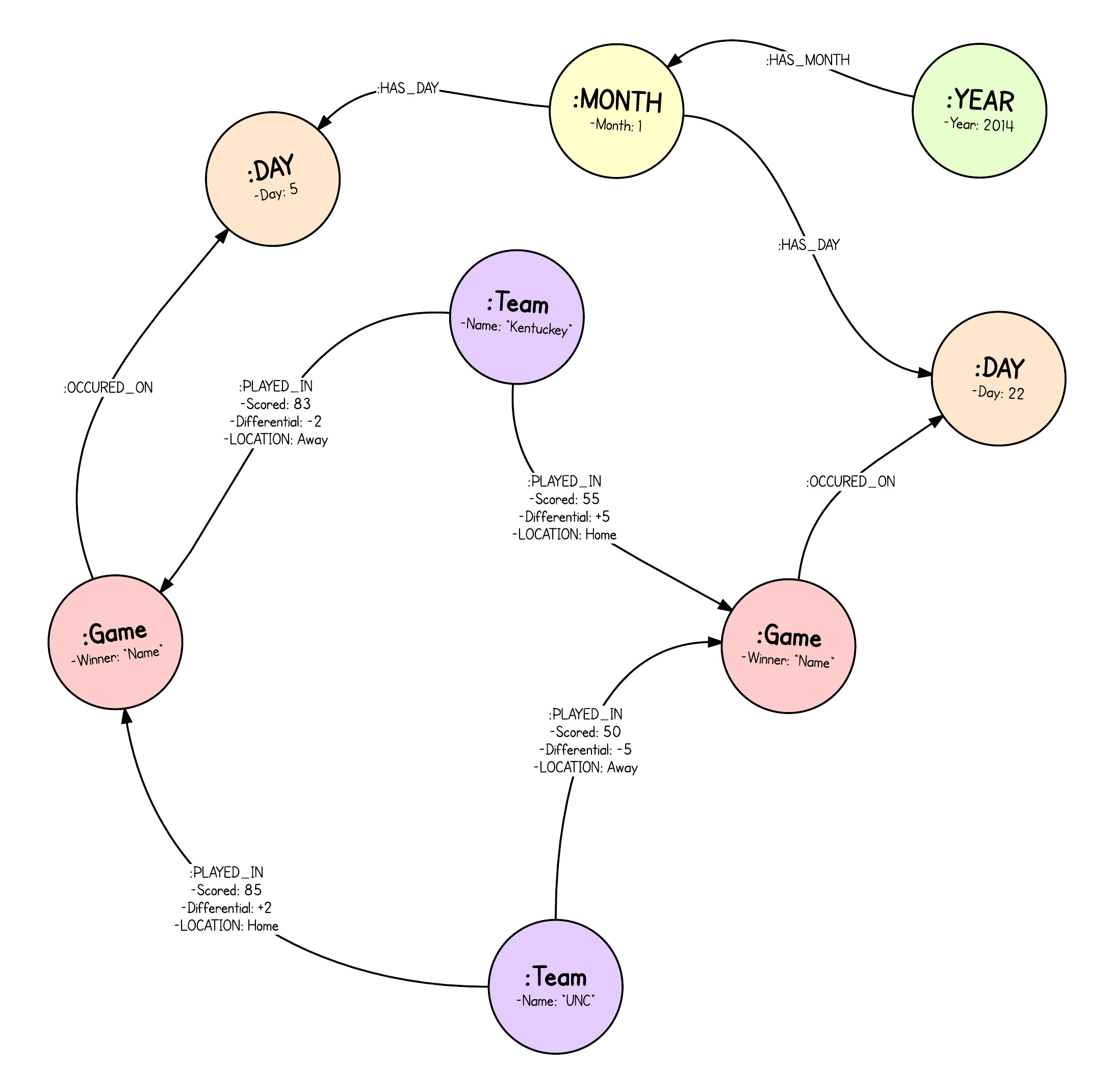
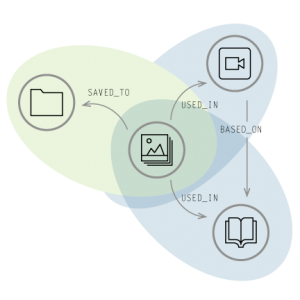
The domain model that interests us here, is pretty straightforward:

(:Person {name}) -[:ACTS_IN|:DIRECTED]-> (:Movie {title})
(:Movie {title}) -[:GENRE]-> (:Genre {name})

HARDWARE

I presume you use a sensible machine, with a SSD (or enough IOPS) and decent amount of RAM. For a highly concurrent load, there should be also enough CPU cores to handle it.

Other questions to consider: Did you monitor io-waits, top, for CPU and memory usage? Any bottlenecks that turn up?

If so, you should address those issues first.

On Linux, configure your disk scheduler to noop or deadline and mount the database volume with noatime. See this blog post for more information.

CONFIG

For best results, use the latest stable version of Neo4j (i.e., Neo4j Enterprise 2.2.5). There is always an Enterprise trial version available to give you a high-watermark baseline, so compare it to Neo4j Community on your machine as needed.

Set dbms.pagecache.memory=4G in conf/neo4j.properties or the size of the store-files (nodes, relationships, properties, string-properties) combined.

ls -lt data/graph.db/neostore.*.db
3802094 16 Jul 14:31 data/graph.db/neostore.propertystore.db
 456960 16 Jul 14:31 data/graph.db/neostore.relationshipstore.db
 442260 16 Jul 14:31 data/graph.db/neostore.nodestore.db
   8192 16 Jul 14:31 data/graph.db/neostore.schemastore.db
   8190 16 Jul 14:31 data/graph.db/neostore.labeltokenstore.db
   8190 16 Jul 14:31 data/graph.db/neostore.relationshiptypestore.db
   8175 16 Jul 14:31 data/graph.db/neostore.relationshipgroupstore.db

Set heap from 8 to 16G, depending on the RAM size of the machine. Also configure the young generation in conf/neo4j-wrapper.conf.

wrapper.java.initmemory=8000
wrapper.java.maxmemory=8000
wrapper.java.additional=-Xmn2G

That’s mostly it, config-wise. If you are concurrency heavy, you could also set the webserver threads in conf/neo4j-server.properties.

# cpu * 2
org.neo4j.server.webserver.maxthreads=24

QUERY TUNING

If these previous factors are taken care of, it’s now time to dig into query tuning. A lot of query tuning is simply prefixing your statements with EXPLAIN to see what Cypher would do and using PROFILE to retrieve the real execution data as well:

For example, let’s look at this query, which has the PROFILE prefix:

PROFILE
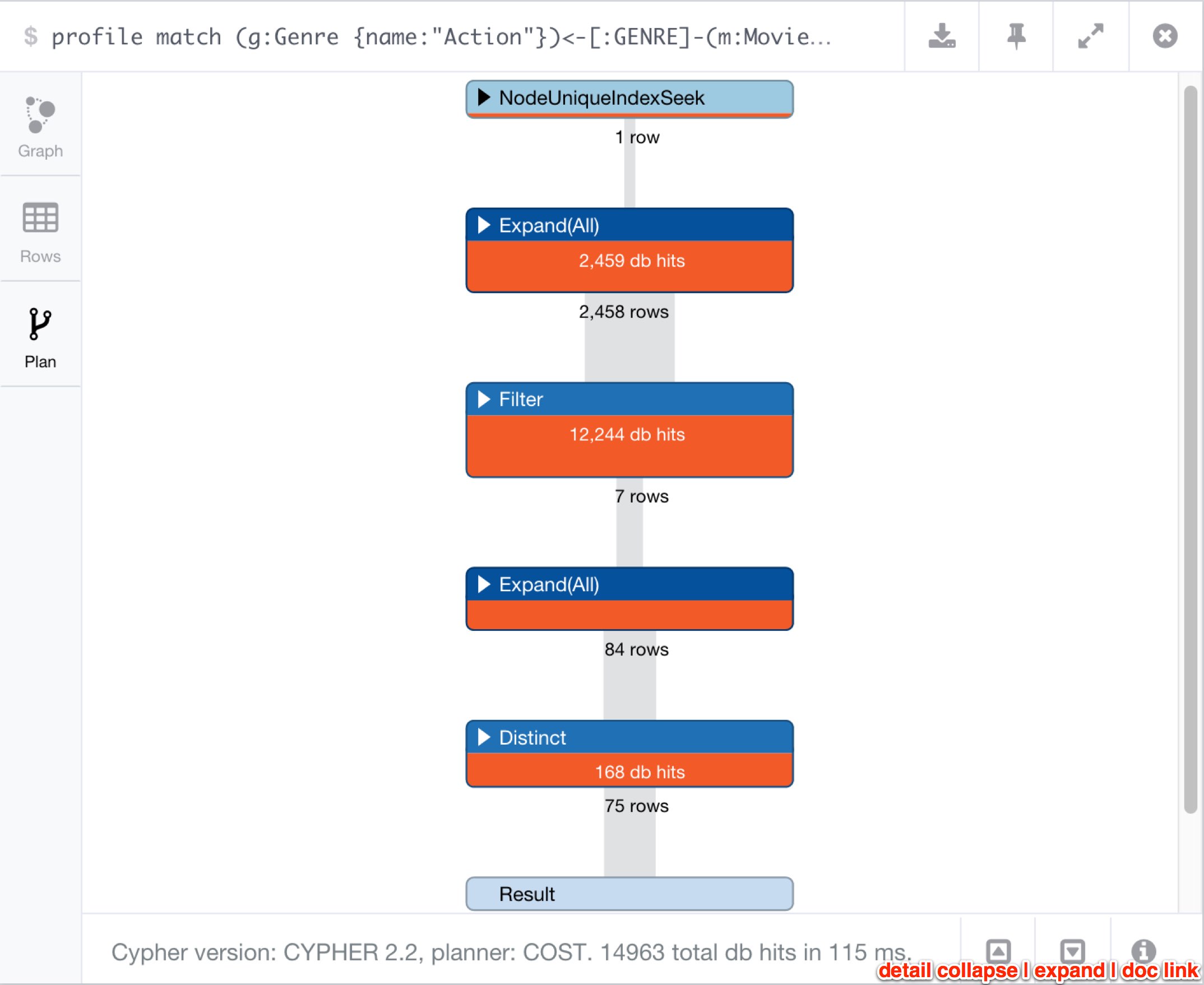
MATCH(g:Genre {name:"Action"})<-[:GENRE]-(m:Movie)<-[:ACTS_IN]-(a)
WHERE a.name =~ "A.*"
RETURN distinct a.name;

The result of this query is shown below in the visual query plan tool available in the Neo4j browser.

A Screenshot of a Query Plan for More Effective Query Tuning

While the visual query plan is nice in the Neo4j browser, the one in Neo4j-shell is easier to compare and it also has more raw numbers.

Operator	Est.Rows	Rows	DbHits	Identifiers	Other
Total database accesses: 72310
Distinct	2048	860	2636	a.name	a.name
Filter(0)	2155	1318	41532	anon[32], anon[52], a, g, m	a.name ~= /{ AUTOSTRING1}/
Expand(All)(0)	2874	20766	23224	anon[32], anon[52], a, g, m	(m)←[:ACTS_IN]-(a)
Filter(1)	390	2458	2458	anon[32], g, m	m:Movie
Expand(All)(1)	390	2458	2459	anon[32], g, m	(g)←[:GENRE]-(m)
NodeUniqueIndexSeek	1	1	1	g	:Genre(name)

Query Tuning Tip #1: Use Indexes and Constraints for Nodes You Look Up by Properties

Check – with either schema or :schema – that there is an index in place for non-unique values and a constraint for unique values, and make sure – with EXPLAIN – that the index is used in your query.

CREATE INDEX ON :Movie(title);
CREATE INDEX ON :Person(name);
CREATE CONSTRAINT ON (g:Genre) ASSERT g.name IS UNIQUE;

Even for range queries (pre-Neo4j 2.3), it might be better to turn them into an IN query to leverage an index.

// if :Movie(released) is indexed, this query for the nineties will *not use* an index:
MATCH (m:Movie) WHERE m.released >= 1990 and m.released < 2000
RETURN count(*);

CREATE INDEX ON :Movie(released);

// but this will
MATCH (m:Movie) WHERE m.released IN range(1990,1999)  RETURN count(*);

// same for OR queries
MATCH (m:Movie) WHERE m.released = 1990 OR m.released = 1991 OR ...

Query Tuning Tip #2: Patterns with Bound Nodes are Optimized

If you have a pattern (node)-[:REL]→(node) where both nodes on either side are already bound, Cypher will optimize the match by taking the node-degree (number of relationships) into account when checking for the connection, starting on the smaller side and also caching internally.

So, for example, (actor)-[:ACTS_IN]->(movie) – if both actor and movie are known – turns into that described Expand(Into) operation.

If one side is not known, then it is a normal Expand(All) operation.

Query Tuning Tip #3: Enforce Index Lookups for Both Sides of a Path

Make sure that if nodes on both sides of a longer path can be found in an index, and are only a few hits of a larger total count, to add USING INDEX for both sides. In many cases, that makes a big difference. It doesn't help if the path explodes in the middle and a simple left-to-right traversal with property checks would touch fewer paths.

PROFILE
MATCH (a:Person {name:"Tom Hanks"})-[:ACTS_IN]->()<-[:ACTS_IN]-(b:Person {name:"Meg Ryan"})
RETURN count(*);

Operator	Est.Rows	Rows	DbHits	Identifiers	Other
Total database accesses: 765
EagerAggregation	0	1	0	count(*)
Filter	0	3	531	anon[36], anon[49], anon[51], a, b	a:Person AND a.name == { AUTOSTRING0}) AND NOT(anon[36] == anon[51]
Expand(All)(0)	3	177	204	anon[36], anon[49], anon[51], a, b	()←[:ACTS_IN]-(a)
Expand(All)(1)	2	27	28	anon[49], anon[51], b	(b)-[:ACTS_IN]→()
NodeIndexSeek	1	1	2	b	:Person(name)

If we add the second index-hint, we get 10x fewer database hits.

PROFILE
MATCH (a:Person {name:"Tom Hanks"})-[:ACTS_IN]->()<-[:ACTS_IN]-(b:Person {name:"Meg Ryan"})
USING INDEX a:Person(name) USING INDEX b:Person(name)
RETURN count(*);

Operator	Est.Rows	Rows	DbHits	Identifiers	Other
Total database accesses: 68
EagerAggregation	0	1	0	count(*)
Filter	0	3	0	anon[36], anon[49], anon[51], a, b	NOT(anon[36] == anon[51])
NodeHashJoin	0	3	0	anon[36], anon[49], anon[51], a, b	anon[49]
Expand(All)(0)	2	27	28	anon[49], anon[51], b	(b)-[:ACTS_IN]→()
NodeIndexSeek(0)	1	1	2	b	:Person(name)
Expand(All)(1)	2	35	36	anon[36], anon[49], a	(a)-[:ACTS_IN]→()
NodeIndexSeek(1)	1	1	2	a	:Person(name)

Query Tuning Tip #4: Defer Property Access

Make sure to access properties only as the last operation – if possible – and on the smallest set of nodes and relationships. Massive property loading is more expensive than following relationships.

For example, this query:

PROFILE
MATCH (p:Person)-[:ACTS_IN]->(m:Movie)
RETURN p.name, count(*) as c
ORDER BY c DESC limit 10;

Operator	Est.Rows	Rows	DbHits	Identifiers	Other
Total database accesses: 404525
Projection(0)	308	10	0	anon[48], anon[54], c, p.name	anon[48]; anon[54]
Top	308	10	0	anon[48], anon[54]	{ AUTOINT0};
EagerAggregation	308	44689	0	anon[48], anon[54]	anon[48]
Projection(1)	94700	94700	189400	anon[48], anon[17], m, p	p.name
Filter	94700	94700	94700	anon[17], m, p	p:Person
Expand(All)	94700	94700	107562	anon[17], m, p	(m)←[:ACTS_IN]-(p)
NodeByLabelScan	12862	12862	12863	m	:Movie

This query shown above accesses p.name for all people, totaling 400,000 database hits. Instead, you should aggregate on the node first, then order and paginate, and only in the very end should you access and return the property.

PROFILE
MATCH (p:Person)-[:ACTS_IN]->(m:Movie)
WITH p, count(*) as c
ORDER BY c DESC LIMIT 10
RETURN p.name, c;

This second query above only accesses p.name for the top ten actors, and before that, it groups them directly by the nodes, saving us about 200,000 database hits.

Operator	Est.Rows	Rows	DbHits	Identifiers	Other
Total database accesses: 215145
Projection	308	10	20	c, p, p.name	p.name; c
Top	308	10	0	c, p	{ AUTOINT0}; c
EagerAggregation	308	44943	0	c, p	p
Filter	94700	94700	94700	anon[17], m, p	p:Person
Expand(All)	94700	94700	107562	anon[17], m, p	(m)←[:ACTS_IN]-(p)
NodeByLabelScan	12862	12862	12863	m	:Movie

But that query could even be optimized more, with....

Query Tuning Tip #5: Fast Relationship Counting

There is an optimal implementation for single path-expressions, by directly reading the degree of a node. Personally, I always prefer this method over optional matches, exists or general where conditions: size((s)-[:REL]->()) ← uses get-degree which is a constant time operation (similarly without rel-type or direction).

PROFILE
MATCH (n:Person) WHERE EXISTS((n)-[:DIRECTED]->())
RETURN count(*);

Here the plan doesn’t count the nested db-hits in the expression, which it should. That’s why I included the runtime:

1 row 197 ms

Operator	Est.Rows	Rows	DbHits	Identifiers	Other
Total database accesses: 106396
EagerAggregation	194	1	56216	count(*)
Filter	37634	6037	0	n	NestedPipeExpression(ExpandAllPipe(….))
NodeByLabelScan	50179	50179	50180	n

versus

PROFILE
MATCH (n:Person) WHERE size((n)-[:DIRECTED]->()) <> 0
RETURN count(*);

1 row 90 ms

Operator	Est.Rows	Rows	DbHits	Identifiers	Other
Total database accesses: 150538
EagerAggregation	213	1	0	count(*)
Filter	45161	6037	100358	n	NOT(GetDegree(n,Some(DIRECTED),OUTGOING) == { AUTOINT0})
NodeByLabelScan	50179	50179	50180	n	:Person

You can also use that technique nicely for overview pages or inline aggregations:

PROFILE
MATCH (m:Movie)
RETURN m.title, size((m)<-[:ACTS_IN]-()) as actors, size((m)<-[:DIRECTED]-()) as directors
LIMIT 10;

+-------------------------------------------------------------+
| m.title                                | actors | directors |
+-------------------------------------------------------------+
| "Indiana Jones and the Temple of Doom" | 13     | 1         |
| "King Kong"                            | 1      | 1         |
| "Stolen Kisses"                        | 21     | 1         |
| "One Flew Over The Cuckoo's Nest"      | 24     | 1         |
| "Ziemia obiecana"                      | 17     | 1         |
| "Scoop"                                | 21     | 1         |
| "Fire"                                 | 0      | 1         |
| "Dial M For Murder"                    | 5      | 1         |
| "Ed Wood"                              | 21     | 1         |
| "Requiem"                              | 11     | 1         |
+-------------------------------------------------------------+
10 rows
13 ms

Operator	Est.Rows	Rows	DbHits	Identifiers	Other
Total database accesses: 71
Projection	12862	10	60	actors, directors,	m.title; GetDegree(m,Some(ACTS_IN),INCOMING);
				m, m.title	GetDegree(m,Some(DIRECTED),INCOMING)
Limit	12862	10	0	m	{ AUTOINT0}
NodeByLabelScan	12862	10	11	m	:Movie

Our query from the previous section would look like this:

PROFILE
MATCH (p:Person)
WITH p, sum(size((p)-[:ACTS_IN]->())) as c
ORDER BY c DESC LIMIT 10
RETURN p.name, c;

This query shaves off another 50,000 database hits. Not bad.

Operator	Est.Rows	Rows	DbHits	Identifiers	Other
Total database accesses: 150558
Projection	224	10	20	c, p, p.name	p.name; c
Top	224	10	0	c, p	{ AUTOINT0}; c
EagerAggregation	224	50179	100358	c, p	p
NodeByLabelScan	50179	50179	50180	p	:Person

Note to self: Optimized Cypher looks more like Lisp.

Bonus Query Tuning Tip: Reduce Cardinality of Work in Progress

When following longer paths, you’ll encounter duplicates. If you’re not interested in all the possible paths – but just distinct information from stages of the path – make sure that you eagerly eliminate duplicates, so that later matches don’t have to be executed many multiple times.

This reduction of the cardinality can be done using either WITH DISTINCT or WITH aggregation (which automatically de-duplicates).

So, for instance, for this query of "Movies that Tom Hanks' colleagues acted in":

PROFILE
MATCH (p:Person {name:"Tom Hanks"})-[:ACTS_IN]->(m1)<-[:ACTS_IN]-(coActor)-[:ACTS_IN]->(m2)
RETURN distinct m2.title;

This query has 10,272 db-hits and touches 3,020 total paths.

Operator	Est.Rows	Rows	DbHits	Identifiers	Other
Total database accesses: 10272
Distinct	4	2021	6040	m2.title	m2.title
Filter(0)	4	3020	0	anon[36], anon[53], anon[75], coActor, m1, m2, p	(NOT(anon[53] == anon[75]) AND NOT(anon[36] == anon[75]))
Expand(All)(0)	4	3388	3756	anon[36], anon[53], anon[75], coActor, m1, m2, p	(coActor)-[:ACTS_IN]→(m2)
Filter(1)	3	368	0	anon[36], anon[53], coActor, m1, p	NOT(anon[36] == anon[53])
Expand(All)(1)	3	403	438	anon[36], anon[53], coActor, m1, p	(m1)←[:ACTS_IN]-(coActor)
Expand(All)(2)	2	35	36	anon[36], m1, p	(p)-[:ACTS_IN]→(m1)
NodeIndexSeek	1	1	2	p	:Person(name)

The first-degree neighborhood is unique, since in this dataset there is only at most one :ACTS_IN relationship between an actor and a movie. So, the first duplicated nodes appear at the second degree, which we can eliminate like this:

PROFILE
MATCH (p:Person {name:"Tom Hanks"})-[:ACTS_IN]->(m1)<-[:ACTS_IN]-(coActor)
WITH distinct coActor
MATCH (coActor)-[:ACTS_IN]->(m2)
RETURN distinct m2.title;

This query tuning technique reduces the number of paths to match for the last step to 2,906. In other use cases with more duplicates, the impact is much bigger.

Operator	Est.Rows	Rows	DbHits	Identifiers	Other
Total database accesses: 9529
Distinct(0)	4	2031	5812	m2.title	m2.title
Expand(All)(0)	4	2906	3241	anon[113], coActor, m2	(coActor)-[:ACTS_IN]→(m2)
Distinct(1)	3	335	0	coActor	coActor
Filter	3	368	0	anon[36], anon[53], coActor, m1, p	NOT(anon[36] == anon[53])
Expand(All)(1)	3	403	438	anon[36], anon[53], coActor, m1, p	(m1)←[:ACTS_IN]-(coActor)
Expand(All)(2)	2	35	36	anon[36], m1, p	(p)-[:ACTS_IN]→(m1)
NodeIndexSeek	1	1	2	p	:Person(name)

Of course we would apply our Minimize Property Access tip here too:

PROFILE
MATCH (p:Person {name:"Tom Hanks"})-[:ACTS_IN]->(m1)<-[:ACTS_IN]-(coActor)
WITH distinct coActor
MATCH (coActor)-[:ACTS_IN]->(m2)
WITH distinct m2
RETURN m2.title;

Operator	Est.Rows	Rows	DbHits	Identifiers	Other
Total database accesses: 7791
Projection	4	2037	4074	m2, m2.title	m2.title
Distinct(0)	4	2037	0	m2	m2
Expand(All)(0)	4	2906	3241	anon[113], coActor, m2	(coActor)-[:ACTS_IN]→(m2)
Distinct(1)	3	335	0	coActor	coActor
Filter	3	368	0	anon[36], anon[53], coActor, m1, p	NOT(anon[36] == anon[53])
Expand(All)(1)	3	403	438	anon[36], anon[53], coActor, m1, p	(m1)←[:ACTS_IN]-(coActor)
Expand(All)(2)	2	35	36	anon[36], m1, p	(p)-[:ACTS_IN]→(m1)
NodeIndexSeek	1	1	2	p	:Person(name)

We still need the distinct m2 at the end, as the co-actors can have played in the same movies, and we don’t want duplicate results.

This query has 7,791 db-hits and touches 2,906 paths in total.

If you are also interested in the frequency (e.g., for scoring), you can compute them along with an aggregation instead of distinctly. In the end, You just multiply the path count per co-actor with the number of occurrences per movie.

MATCH (p:Person {name:"Tom Hanks"})-[:ACTS_IN]->(m1)<-[:ACTS_IN]-(coActor)
WITH coActor, count(*) as freq
MATCH (coActor)-[:ACTS_IN]->(m2)
RETURN m2.title, freq * count(*) as occurrence;

Conclusion

The best way to start with query tuning is to take the slowest queries, PROFILE them and optimize them using these tips.

If you need help, you can always reach out to us on Stack Overflow, our Google Group or our public Slack channel.

If you are part of a project that is adopting Neo4j or putting it into production, make sure to get some expert help to ensure you’re successful. Note: If you do ask for help, please provide enough information for others to be able to help you. Explain your graph model, share your queries, their profile output and – best of all – a dataset to run them on.

Need more tips on how to effectively use Neo4j? Register for our online training class, Neo4j in Production, and learn how to master the world’s leading graph database.

Sign Me Up

↧

Graph Databases in the Enterprise: Graph-Based Search

November 9, 2015, 4:00 am

≫ Next: How Backstory.io Uses Neo4j to Graph the News [Community Post]

≪ Previous: 5 Secrets to More Effective Neo4j 2.2 Query Tuning

Learn More about the Graph-Based Search Use Case of Graph Databases in the Enterprise

Graph-based search is a new approach to data and digital asset management originally pioneered by Facebook and Google.

Search powered by a graph database delivers relevant information that you may not have specifically asked for – offering a more proactive and targeted search experience, allowing you to quickly triangulate the data points of the greatest interest.

The key to this enhanced search capability is that on the very first query, a graph-based search engine takes into account the entire structure of available connected data. And because graph systems understand how data is related, they return much richer and more precise results.

Think of graph-based search more as a “conversation” with your data, rather than a series of one-off searches. It’s search and discovery, rather than search and retrieval.

In this “Graph Databases in the Enterprise” series, we’ll explore the most impactful and profitable use cases of graph database technologies at the world’s leading organizations. In past weeks, we’ve examined fraud detection, real-time recommendation engines, master data management, network & IT operations and identity & access management (IAM).

This week, we’ll take a closer look at graph-based search.

The Key Challenges in Graph-Based Search:

As a cutting edge technology, graph-based search is beset with challenges. Here are some of the biggest:

The size and connectedness of asset metadata

Real-time query performance

power of a graph-based search application

Growing number of data nodes

Why Use a Graph Database for Graph-Based Search?

Graph-based search would be impossible without a graph database to power it.

In essence, graph-based search is intelligent: You can ask much more precise and useful questions and get back the most relevant and meaningful information, whereas traditional keyword-based search delivers results that are more random, diluted and low-quality.

With graph-based search, you can easily query all of your connected data in real time, then focus on the answers provided and launch new real-time searches prompted by the insights you’ve discovered.

Graph databases make advanced search-and-discovery possible because:

Enterprises can structure their data exactly as it occurs and carry out searches based on their own inherent structure. Graph databases provide the model and query language to support the natural structure of data.
Users receive fast, accurate search results in real time. With a graph database, a variety of rich metadata is assigned to all content for rapid search and discovery.
Data architects and developers can easily change their data and its structure as well as add a wide variety of new data. The built-in flexibility of a graph database model allows for agile changes to search capabilities.

In contrast, information held in a relational database is much more inflexible to future change: If you want to add new kinds of content or make structural changes, you are forced to re-work the relational model in a way that you don’t need to do with the graph model.

The graph model is much more easily extensible and over 1,000 times faster than a relational database when working with connected data.

Example: Google and Facebook

In their early days, both Facebook and Google offered a basic “keyword” search, where users would type in a word or phrase and get back a list of all results that included those keywords.

This method relied on plain pattern recognition, and many users found it to be a cumbersome process of repeatedly redefining search terms until the correct result was found.

Facebook’s database of people and Google’s database of information have one crucial thing in common: They were both built using graph technology. And in recent years, both Google and Facebook have realized they could make much better use of their huge swathes of searchable content, and have each launched new graph-based search services to exploit these commercial opportunities.

Realizing the limitations of keyword searches, Google launched its “Knowledge Graph” in 2012 and Facebook followed suit with its “Graph Search” service in 2013, both of which provide users with more contextual information in their searches.

As a result of these new services, both enterprises realized substantial lift in user engagement – and therefore commercial success.

Following in the footsteps of giants like Facebook, Google and adidas, new startups like Glowbl and Decibel – and many others – have also created graph-based search tools to discover new business insights, launch new products and services and attract new customers.

Conclusion

For businesses that have huge volumes of products, content or digital assets, graph-based search provides a better way to make this data available to users, as corporate giants Google and Facebook have clearly demonstrated.

The valuable uses of graph-based search in the enterprise are endless; customer support portals, product catalogs, content portals and social networks are just a few.

Graph-based search offers numerous competitive advantages, including better customer experience, more targeted content and increased revenue opportunities.

Enterprises that tap into the power of graph-based search today will be well ahead of their peers tomorrow.

Download your copy of this white paper, The Top 5 Use Cases of Graph Databases, and discover how to tap into the power of connected data at your enterprise.

Download the White Paper

Catch up with the rest of the “Graph Databases in the Enterprise” series:

Fraud Detection

Real-Time Recommendation Engines

Master Data Management

Network and IT Operations

Identity and Access Management

Enterprise Competitive Advantage

↧

How Backstory.io Uses Neo4j to Graph the News [Community Post]

December 1, 2015, 4:00 am

≫ Next: Non-Text Discovery with ConceptNet as a Neo4j Database [Community Post]

≪ Previous: Graph Databases in the Enterprise: Graph-Based Search

[As community content, this post reflects the views and opinions of the particular author and does not necessarily reflect the official stance of Neo4j.]

Backstory is a news exploration website I co-created with my friend Devin.

The site automatically organizes news from hundreds of sources into rich, interconnected timelines. Our goal is to empower people to consume news in a more informative and open-ended way.

The News Graph

Our ability to present and analyze news in interesting ways is based on an extensive and ever-growing “news graph” powered by Neo4j.

The core graph model is shown in simplified form below:

Consider three articles published by different news sources on November 16th, 2015.

First, Backstory collects these articles and stores them as ARTICLE nodes in the graph.

Second, article text is analyzed for named entities, stored as ACTOR nodes. Articles have a REFERENCED relationship with their actors.

Thirdly, these articles are clustered because they’re about the same thing: U.S. Secretary of State John Kerry visiting France after the terrorist attacks in Paris. The article cluster is represented by an EVENT node. All articles and actors in a cluster point to their news event with an IN_EVENT relationship.

Finally, all actors in the cluster point to one another using a dated WITH relationship, to record their co-occurrence.

Given enough data, this model allows us to answer interesting questions about the news with simple Cypher queries. For example:

What are the most recent news events involving John Kerry?

MATCH (:ACTOR {name: "John Kerry"})-[:IN_EVENT]-(e:EVENT) RETURN e ORDER BY e.date DESC LIMIT 10

When was the last time Islamism interacted with Paris?

MATCH (:ACTOR {name: "Islamism"})-[w:WITH]-(:ACTOR {name: "Paris"}) RETURN w.date ORDER BY w.date DESC LIMIT 1

How many news events involving France occurred this week?

MATCH (:ACTOR {name: "France"})-[:IN_EVENT]-(e:EVENT) WHERE e.date > 1447215879786 RETURN count(e) AS event_count

In addition to the information present in the news graph itself, we tap into a large amount of enriched data by virtue of correlating all actor nodes to Wikipedia entries.

For example, by including a field about the type of thing an actor is, a query can now differentiate a person from a place. Cypher has risen to the challenge and continues to allow for concise queries over a complexifying graph.

Neo4j For The Win

We are big Neo4j fans at Backstory. The graph technology and community has propelled us forward in many ways.

Here are just a few examples:

There Are Ample Neo4j Clients across Languages

In the Backstory system architecture – described in more detail here – there are a variety of components that read from and write to the graph database.

A combination of requirements and personal taste have led us to write these components in different languages, and we are pleased with the variety of options available for talking to Neo4j.

On the write-side, we use the the Neo4j Java REST Bindings. This component also uses a custom testing framework that allows us to run suites of integration tests against isolated, transient Neo4j embedded instances.

On the read-side, we’ve created an HTTP API that has codified the queries the Backstory.io website makes. This is written in Python and uses py2neo.

There’s also an ExpressJS API for administrative purposes, which constructs custom Cypher queries and manages its own transactions with Neo4j.

The Neo4j Browser Is a Crucial Experimentation Tool

The Neo4j Browser is an excellent tool for anything from experimenting with new Cypher queries to running some sanity checks on your production data.

Every Cypher-based feature I’ve developed for Backstory was conceived and hardened in the Browser. I even used it to develop the example queries above!

Graph Flexibility Is Underrated

Early on in our design process for Backstory we were a bit skeptical of using a graph database. Was it really worth leaving the comfort zone of relational databases or key-value stores?

Even after we had committed to a Neo4j prototype, we expected to end up requiring secondary relational storage for any number of requirements outside of the core news graph.

It turns out Neo4j has sufficed for all of our persistent data requirements, and has even led us to novel solutions in several cases. Four quick examples:

Ability to latently add indexes

Using Neo4j as an article queue

Using the graph to cluster articles

Using Neo4j for Named Entity recognition

Conclusion

As mentioned above, our goal with Backstory is to create better ways for people to consume news and understand the world. Part of this is having a world-class technology platform for collecting and analyzing news.

Neo4j’s vibrant community and the flexibility of the graph database are enabling us to achieve these goals.

Instead of thinking about our database simply as a place where bits are stored, we think of our data as alive and brimming with insights. The graph lets our data breathe, striking the right balance between structure and versatility. Meanwhile, Cypher queries continue to perform well as the model grows more complex.

The Neo4j-powered news graph is absolutely the centerpiece of our system, and we’re excited for what the future holds.

If you’d like to follow our progress, join the mailing list on http://backstory.io or give us a follow on Twitter at @backstoryio.

Ready to use Neo4j for your next app or project? Get everything you need to know about harnessing graphs in O’Reilly’s Graph Databases – click below to get your free copy.

Get My Free Copy

↧

Non-Text Discovery with ConceptNet as a Neo4j Database [Community Post]

January 21, 2016, 4:00 am

≫ Next: 3 RDBMS & Graph Database Deployment Strategies (Polyglot & More)

≪ Previous: How Backstory.io Uses Neo4j to Graph the News [Community Post]

[As community content, this post reflects the views and opinions of the particular author and does not necessarily reflect the official stance of Neo4j.]

The Problem of Discovery

Discovery, especially non-text discovery, is hard.

When looking for a cool T-shirt, for example, I might not know exactly what I want, only that I’m looking for a gift T-shirt that’s a little mathy that emphasizes my friend’s love of nature.

As a retailer, I might notice that geometric nature products are quite popular, and want to capitalize by marketing the more general “math/nature” theme to potential buyers who have demonstrated an affinity for mathy animal shirts as well as improving the browsing experience for new visitors to my site.

Many retail sites with user-generated content rely on user-generated tags to classify image-driven products. However, the quality and number of tags on each item vary widely and depend on the item’s creator and the administrators of the site to curate and sort into browsable categories.

On Threadless, for example, this awesome item has a rich amount of tags:

lim heng swee, ilovedoodle, cats, lol, funny, humor, food, foodies, food with faces, pets, meow, ice cream, desserts,awww, puns, punny, wordplay, v-necks, vnecks, tanks, tank tops, crew sweatshirts, Cute

In contrast, this beautiful item has only a handful:

jimena salas, jimenasalas, funded, birds, animals, geometric shapes, abstract, Patterns

Furthermore, although a human might easily be able to classify an image with the tags [ants, anthill, abstract, goofy] as probably belonging to the “funny animals” category, an automated system would have to know that ants are animals and that goofy is a synonym for funny.

Knowing this, how would a retail site quickly and cheaply implement intelligent categorization and tag curation? ConceptNet5 and (of course), Neo4j.

ConceptNet5

This article introduces the ConceptNet dataset and describes how to import the data into a Neo4j database.

To paraphrase the ConceptNet5 website, ConceptNet5 is a semantic network built from nodes representing words or short phrases of natural language (“terms” or “concepts”), and the relationships (“associations”) between them.

Armed with this information, a system can take human words as input and use them to better search for information, answer questions and understand user goals.

For example, take a look at toast in the ConceptNet5 web demo:

This looks remarkably similar to a graph model. The dataset is incredibly rich, including (in the JSON) the “sense” of toast as a bread and also as a drink one has in tribute.

Let’s take a look at the JSON response for one ConceptNet edge (the association between two concepts) and import some data into a Neo4j database for exploration:

{
     edges: 
     [
          {
               context: "/ctx/all",
               dataset: "/d/globalmind",
               end: "/c/en/bread",
               features: 
               [
                    "/c/en/toast /r/IsA -",
                    "/c/en/toast - /c/en/bread",
                    "- /r/IsA /c/en/bread"
               ],
               id: "/e/ff9b268e050d62255f236f35ba104300551b8a3b",
               license: "/l/CC/By-SA",
               rel: "/r/IsA",
               source_uri:                                              
               "/or/[/and/[/s/activity/globalmind/assert/,/s/
               contributor/omcs/bugmenot/]/,/s/umbel/2013/]",
               sources: 
               [
                    "/s/activity/globalmind/assert",
                    "/s/contributor/omcs/bugmenot",
                    "/s/umbel/2013"
               ],
               start: "/c/en/toast",
               surfaceText: "Kinds of [[bread]] : [[toast]]",
               uri: "/a/[/r/IsA/,/c/en/toast/,/c/en/bread/]",
               weight: 3
          },
}

Modeling the Database

For the purposes of this example, let’s model the database to have the following properties: Term Nodes:

concept
language
partOfSpeech
sense

Association Relationships:

type
weight
surfaceText

An alternate model could have “type” be the relationship label instead of a property, but for the sake of this blog post let’s keep types as properties. This allows us to explore the ConceptNet database without making assumptions about the types of relationships in the dataset.

Loading the Data into the Database

Let’s use the following Python script to upload some sample data:

import requests
import json
from py2neo import authenticate, Graph
 
USERNAME = "neo4j" #use your actual username
PASSWORD = "12345678" #use your actual password
authenticate("localhost:7474", USERNAME, PASSWORD)  
graph = Graph()

#sample_tags = ['fruit','orange','bikes','cream','nature', 'toast','electronic', 'techno', 'house', 'dubstep', 'drum_and_bass', 'space_rock', 'psychedelic_rock', 'psytrance', 'garage', 'progressive','Cologne', 'North_Rhine-Westphalia', 'gothic_rock', 'darkwave' 'goth', 'geometric', 'nature', 'skylines', 'landscapes', 'mountains', 'trees', 'silhouettes', 'back_in_stock', 'Patterns', 'raglans','giraffes', 'animals', 'nature', 'tangled', 'funny', 'cute', krautrock]

# Build query.
query = """
WITH {json} AS document
UNWIND document.edges AS edges
WITH 
SPLIT(edges.start,"/")[3] AS startConcept,
SPLIT(edges.start,"/")[2] AS startLanguage,
CASE WHEN SPLIT(edges.start,"/")[4] <> "" THEN SPLIT(edges.start,"/")[4] ELSE "" END AS startPartOfSpeech,
CASE WHEN SPLIT(edges.start,"/")[5] <> "" THEN SPLIT(edges.start,"/")[5] ELSE "" END AS startSense,
SPLIT(edges.rel,"/")[2] AS relType,
CASE WHEN edges.surfaceText <> "" THEN edges.surfaceText ELSE "" END AS surfaceText,
edges.weight AS weight,
SPLIT(edges.end,"/")[3] AS endConcept,
SPLIT(edges.end,"/")[2] AS endLanguage,
CASE WHEN SPLIT(edges.end,"/")[4] <> "" THEN SPLIT(edges.end,"/")[4] ELSE "" END AS endPartOfSpeech,
CASE WHEN SPLIT(edges.end,"/")[5] <> "" THEN SPLIT(edges.end,"/")[5] ELSE "" END AS endSense
MERGE (start:Term {concept:startConcept, language:startLanguage, partOfSpeech:startPartOfSpeech, sense:startSense})
MERGE (end:Term  {concept:endConcept, language:endLanguage, partOfSpeech:endPartOfSpeech, sense:endSense})
MERGE (start)-[r:ASSERTION {type:relType, weight:weight, surfaceText:surfaceText}]-(end)
"""

# Using the Search endpoint to load data into the graph
for tag in sample_tags:
	searchURL = "http://conceptnet5.media.mit.edu/data/5.4/c/en/" + tag + "?limit=500"
	searchJSON = requests.get(searchURL, headers = 
	{"accept":"application/json"}).json()
	graph.cypher.execute(query, json=searchJSON)

Exploring the Data

Use the following Cypher query to explore the data:

MATCH (n:Term {language:'en'})-[r:ASSERTION]->(m:Term {language:'en'})
WHERE 
NOT r.type = 'dbpedia' AND
NOT r.surfaceText = '' AND
NOT n.partOfSpeech = '' AND
NOT n.sense = ''
RETURN n.concept AS `Start Concept`, n.sense AS `in the sense of`, r.type, m.concept AS `End Concept`, m.sense AS `End Sense`
ORDER BY r.weight DESC, n.sense ASC
LIMIT 10

The ConceptNet dataset is incredibly rich, providing various “senses” in which someone might mean “orange” and provides a wide variety of “relationship types” to choose from.

    | Start Concept | in the sense of                                         | r.type     | End Concept     | End Sense
----+---------------+---------------------------------------------------------+------------+-----------------+-----------
  1 | orange        | colour                                                  | IsA        | color           |
  2 | orange        | film                                                    | InstanceOf | film            |
  3 | dynamic       | a_characteristic_or_manner_of_an_interaction_a_behavior | Synonym    | nature          |
  4 | garage        | a_petrol_filling_station                                | Synonym    | petrol_station  |
  5 | garage        | a_petrol_filling_station                                | Synonym    | fill_station    |
  6 | garage        | a_petrol_filling_station                                | Synonym    | gas_station     |
  7 | progressive   | advancing_in_severity                                   | Antonym    | non_progressive |
  8 | shop          | automobile_mechanic's_workplace                         | Synonym    | garage          |
  9 | electronic    | band                                                    | IsA        | band            |
 10 | cream         | band                                                    | IsA        | band            |

Use Cases and Future Directions

When translated into a graph database, the ConceptNet5 API takes the agony out of tag-based recommendations and categorizations.

Small retail and social startups can integrate a Neo4j microservice into their currently existing stack, using it to power recommendations, provide insights on what is the most effective way to categorize products (should “funny cats” have their own first-level category, or should they go under “animals”?), and allow more time and budget for richer innovations.

References

Loading JSON into a Neo4j Database

Dealing with Empty Columns

Data

ConceptNet5 (thanks to Marvin Minsky, Luminoso, Push Singh and the MIT Media Lab)
WordNet

Learn how to build a real-time recommendation engine for non-text discovery on your website: Download this white paper – Powering Recommendations with a Graph Database – and start offering more timely, relevant suggestions to your users.

Get the White Paper

↧

Talk to us about how you guys use Neo4j at CluedIn.

What made you choose Neo4j?

Can you talk to me about some of your most interesting or surprising results you’d had while using Neo4j?

If you could start over with Neo4j, taking everything you know now, what would you do differently?

What do you think the future of graph technology looks like in your industry or sector?

Anything else you want to add or say?

Talk to us about how you guys use Neo4j at eBay.

You’ve been using Neo4j a while, right?

What made you choose Neo4j?

What do you think the future of graph technology looks like?

Presentation Summary

Full Presentation: Decyphering Your Graph Model

Building Your Model Using Natural Language

Building a Natural Language Model in Your Domain

From Model to Graph

Diving Into Cypher

Conclusion

Conclusion

About Graph Algorithms in Practice

Graph Model

Data Import

Exploratory Data Analysis

Trip Planning

Finding Influential Hotel Reviewers

Finding Similar Categories

Conclusion

Third Prize

Second Prize

First Prize

GraphGists evolving & The next GraphGist Challenge

To be honest, we were blown away.

Education

Finance

Life Science

Manufacturing

Sports

Resources

Retail

Telecommunication

Transport

Advanced Graph Gists

Other

Celebrate American independence and freedom from table structures with these four blog posts.

Happy Fourth of July and happy graphDB reading from the Neo4j team!

Articles

Graphgists

Videos

OSCON Twitter Graph

Graph Visualization

Neo4j Co-Founder and GraphConnect speaker discusses the role of Graph databases in the future of finance

Applying Dating Insights to the Financial Sector

The ‘Social Network’ Analysis

GraphConnect 2014

Watch the Webinar:

March GRAPHness

It’s All Relative

STEP 1: Idea —> Graph Model

STEP 2: Time

STEP 3: my.csv —> graph.db

STEP 4: History, Victory and a Little Math

STEP 5: The Big Payout

Introducing JCypher

Business Domains

Domain Queries

Generic Graph Model

Native Java Domain-Specific Language

Can you tell me a little bit more about you and your organization?

Can you share more specifically how you view those advantages?

Can you tell me a little more about the requirements of the deployment you did for a large telecommunications provider?

How did you get involved?

How many people were there on the Proof of Concept Team? And how did the deployment evolve?

What were some of the other benefits that the Neo4j deployment achieved there?

HARDWARE

CONFIG

QUERY TUNING

Query Tuning Tip #1: Use Indexes and Constraints for Nodes You Look Up by Properties

Query Tuning Tip #2: Patterns with Bound Nodes are Optimized

Query Tuning Tip #3: Enforce Index Lookups for Both Sides of a Path

Query Tuning Tip #4: Defer Property Access

Query Tuning Tip #5: Fast Relationship Counting